3.4. EHF Finger With Constant Plasma Heat Flux

In this tutorial one can understand on how to create basic Elmer case with the help of Elmer toolbox, that is included into Elmer module. BREP file of EHF finger will be imported into SMITER GUI and then appropriately modified and meshed. Then the user will learn how to define material properties and boundary conditions and assign them to the mesh. In the end the computation will be run and results will be shown in the Paraview module.

3.4.1. Importing BREP file into SMITER GUI

To import BREP file to SMITER GUI, first activate Geometry module, as shown in figure Fig. 3.23.

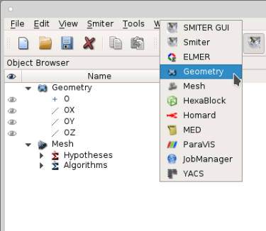
Fig. 3.23 Select GEOM option to activate geometry module.

Then navigate to file File ‣ import ‣ BREP, as shown in figure Fig. 3.24

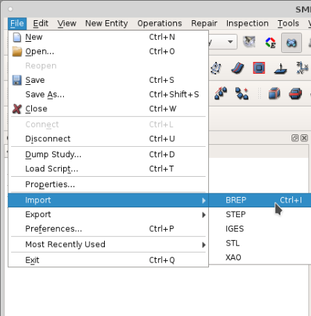
Fig. 3.24 To import BREP file, go to File ‣ import ‣ BREP.

Then navigate to the appropriate folder with the EHF finger and click Open. Refer to figure Fig. 3.25.

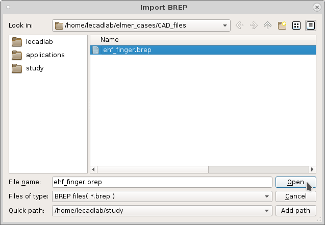
Fig. 3.25 To open the BREP file, navigate to its directory, select the file and click Open.

The imported BREP file is shown in the object browser under Geometry section. The CAD model is displayed in the OCC viewer on the right side.

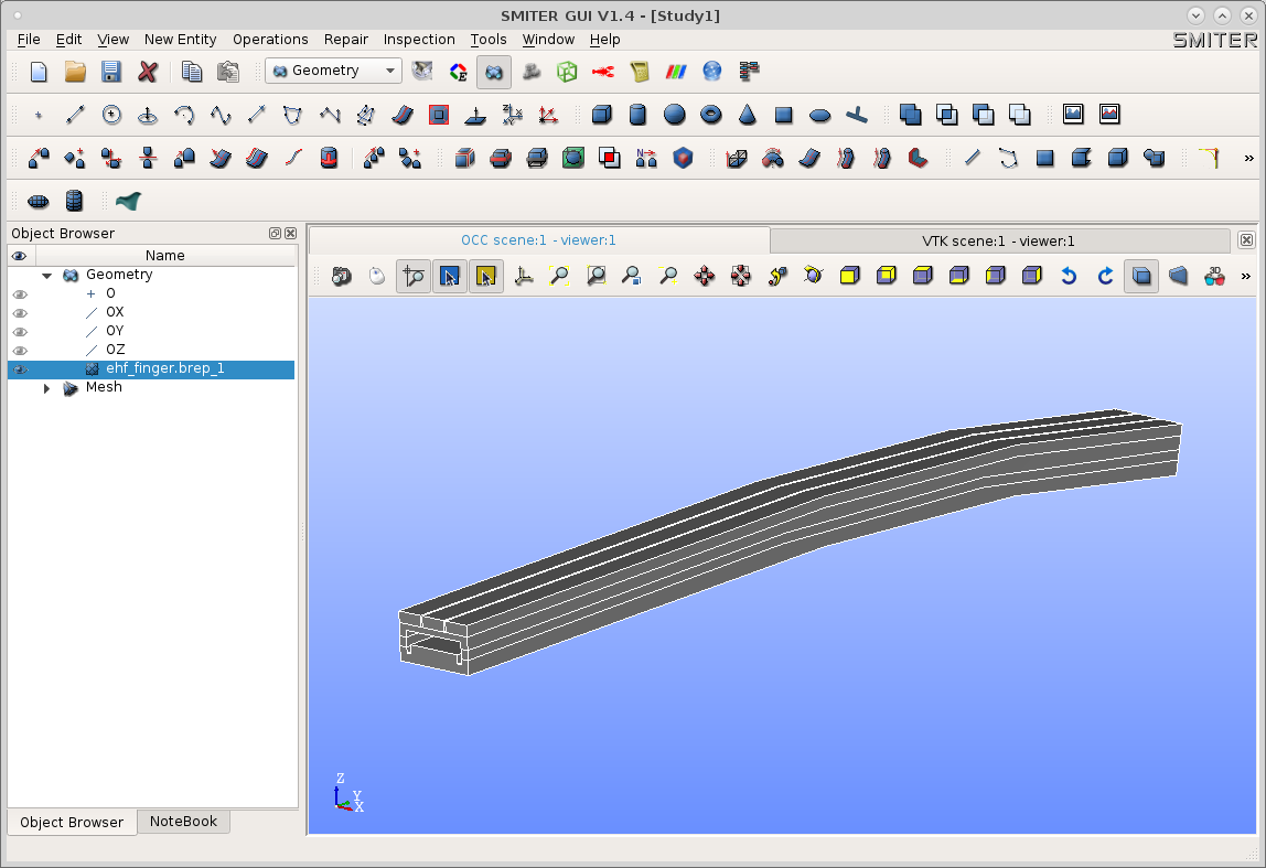
Fig. 3.26 After BREP import the CAD file is seen in the Object Browser and OCC viewer.

3.4.2. Defining Subsections

Now we have to divide the model into different subsections. Those subsection have their own independent properties like boundary conditions and material properties. In this tutorial we have three boundary conditions. On top of the finger is constant heat flux due to plasma. In the tank there is cooling temperature of water and heat transfer coefficient. Other areas around the finger are adiabatic. There are also three main components with different material properties, that need to be defined as well. Refer to figure Fig. 3.6.

To define subsections, we have to break down the CAD model to basic entities (like faces, edges, etc) and then merge them back together to get the appropriate subsection. First select the CAD object in Object Browser. Then navigate to New Entity ‣ Explode. Refer to figure Fig. 3.27. With this option the user can break the whole CAD model down to multiple different geometrical entities.

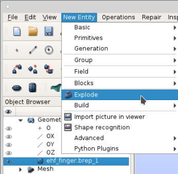
Fig. 3.27 To explode CAD model into its subcomponents, navigate to New Entity ‣ Explode.

After Explode option is selected, the dialog in figure Fig. 3.28 appeares on the screen.

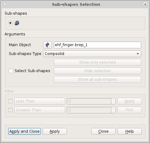
Fig. 3.28 Dialog to select subshapes of CAD model.

Here user user must first select the main object that will be exploded. The user can select the object in the Object Browser in Geometry section. The possible sub-shapes types are shown in figure Fig. 3.29.

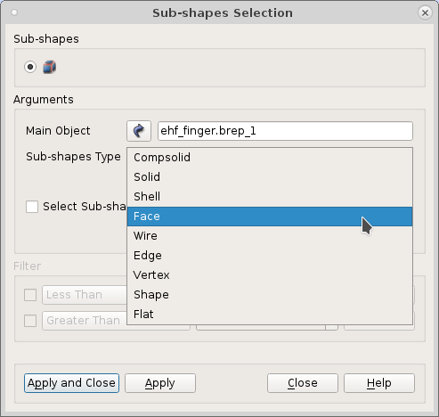
Fig. 3.29 Selection of sub-shapes type.

The defined problem is three-dimensional, thus the boundary conditions will be defined on faces and material properties on solids. In Sub-shapes type combo box select Face option and then click Apply. Repeat the same step for Solid option and then click Apply and Close. After that move to the Object Browser and right click on the object that was just exploded to faces and solids. Select option Expand All. All geometrical entities of selected subshape type in the main model will be displayed in the Object Browser. See figure Fig. 3.30.

Now the user can join two or mode geometrical entites into a group, that presents the subsection. To do that, right click on the main model in Object browser and then select Create Group. See figure Fig. 3.30.

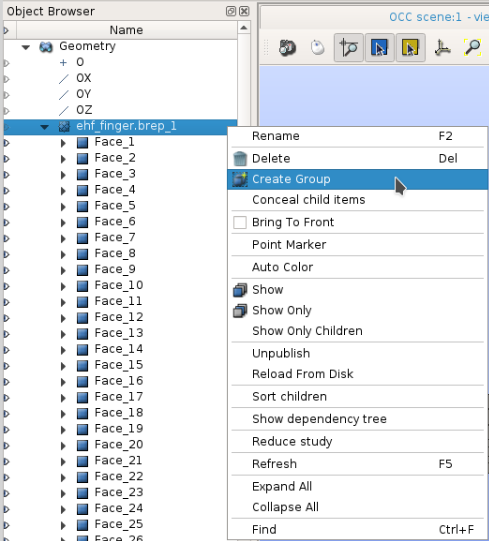
Fig. 3.30 To create group out of child substructures of the parent structure, right click on the object in Object Browser and click Create Group.

The dialog in figure Fig. 3.31 appeares on screen.

Fig. 3.31 Dialog to create groups. The group can contain only one tybe of subshape (vertex, edges and wires, faces and solids).

In this dialog one must first select the shape type of entites that will be included into group. The basic entities are vertices (0D), edges (1D), faces (2D) and solids (3D). Next one must define the group name and the main shape. Then the user can select the entities. The default option for the restriction of selection is No restriction.The entities can be selected interactively in the OCC Viewer. The user can hover over the entity in the viewer with the mouse pointer and the entity edges will turn blue. See figure Fig. 3.32.

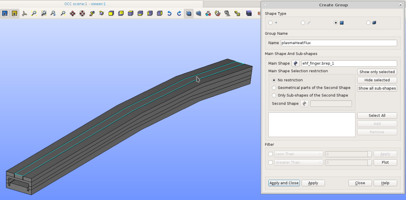
Fig. 3.32 Hover over faces and click left mouse button to add them to group.

If the user click on it, the face edges will turn white and this means that the face was selected. Then the user can move back to dialog and select Add. See figure Fig. 3.33. ID number of the added entity is shown in the left dialog. This way the user cad add different entities to the group. To select more entities, hold down Shift key. After the selection is complete, one can click Apply and Close.

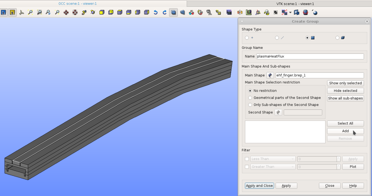
Fig. 3.33 Dialog to create groups from existing CAD models.

The user has to repeat this step for every subsection. Three subcomponents that define boundary condition regions, are shown in figure Fig. 3.34.

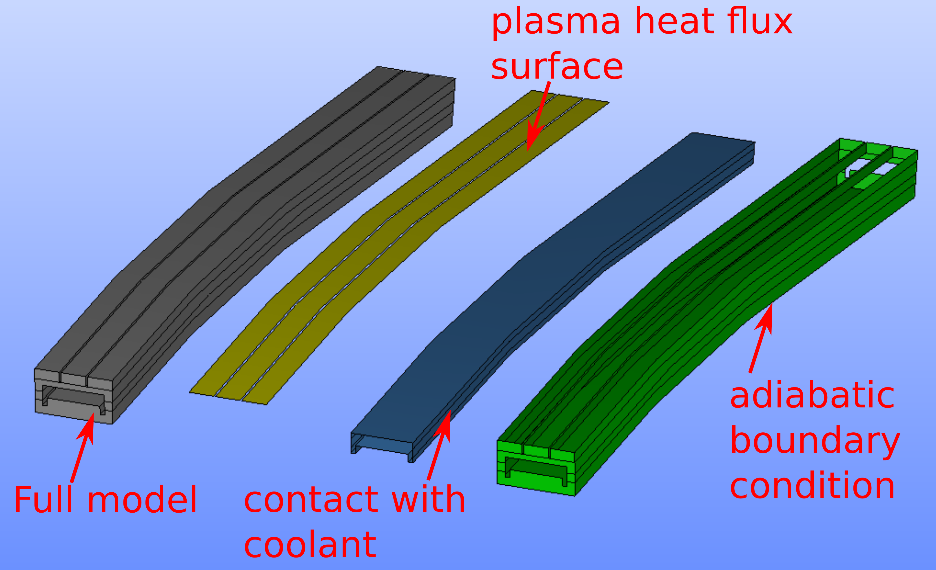
Fig. 3.34 Selection of surfaces to define groups that will present boundary conditions.

Same step has to be repeated for solids. Refer to figure Fig. 3.6 to see the different definitions of materials and sections. All solid subsections are shown in figure Fig. 3.35.

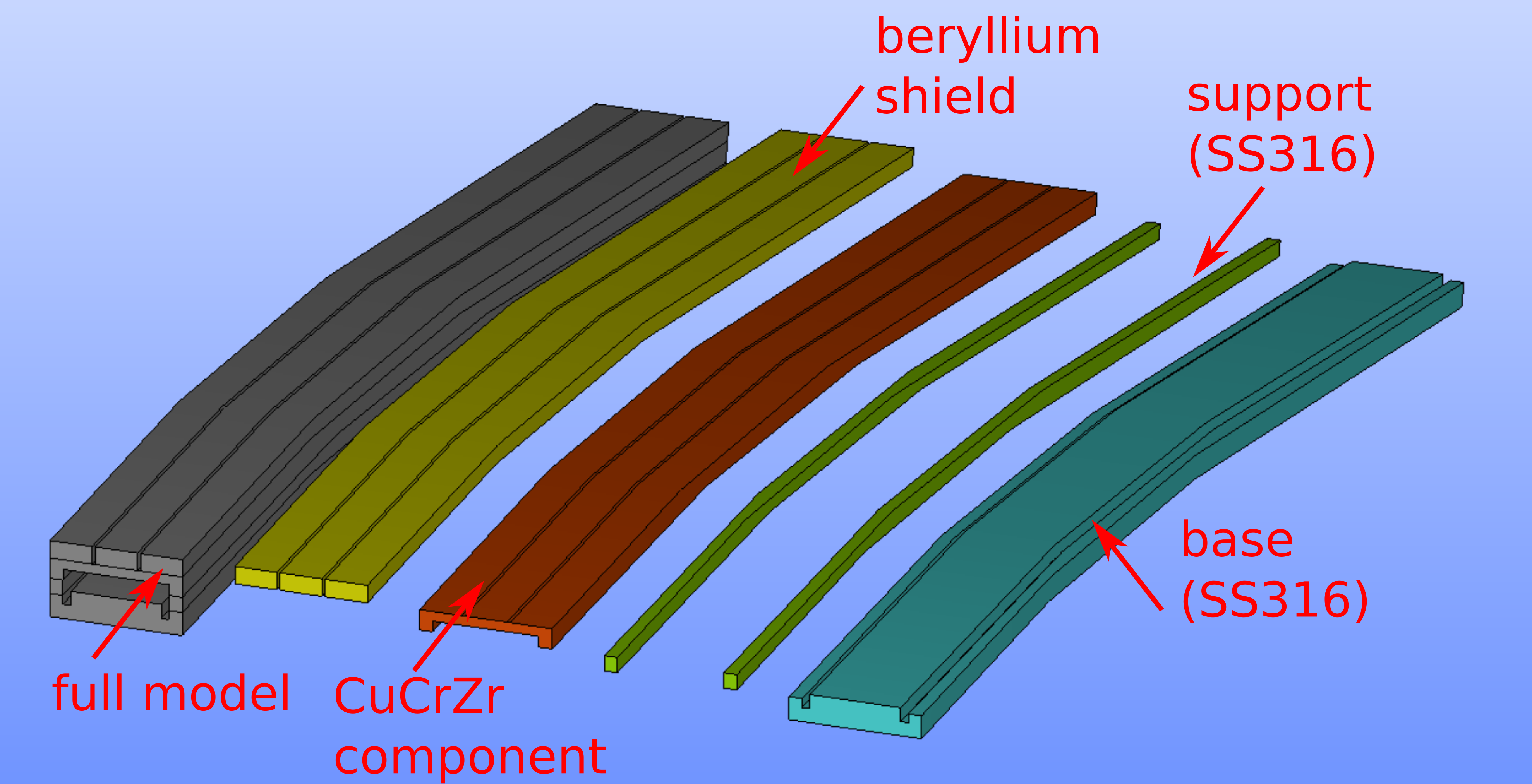
Fig. 3.35 Selection of solids to define groups that will present different materials used in the case.

All newly defined groups can be seen in Object browser under the main object. See figure Fig. 3.36.

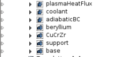
Fig. 3.36 Newly defined groups.

3.4.3. Meshing the CAD model

After all of the subsections of CAD model were defined, the user can move to Mesh module. To activate mesh module, click on Mesh in the combo box option. See figure Fig. 3.37.

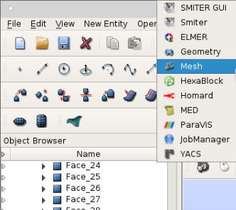
Fig. 3.37 Activate SMESH module to create and manipulate meshes.

To mesh the finger, the user must first select it in the Object browser and then go to Mesh ‣ Create Mesh. New dialog appeares on the screen. Refer to figure Fig. 3.38. First the user can type new mesh name, following the selection of the CAD object that the user wants to mesh. Then the user can specify the prarameters for the hypotheses, algorithms and type of mesh. There are many possible options and the user can decide for himself what kind of mesh he wants to generate. In this tutorial automatic tetrahedralization is specified with the approximate length of edge of the tetrahedron of 0.01 \(mm\). To get more detailed informations on how to mesh CAD models in SMITER GUI, refer to section Meshing CAD models.

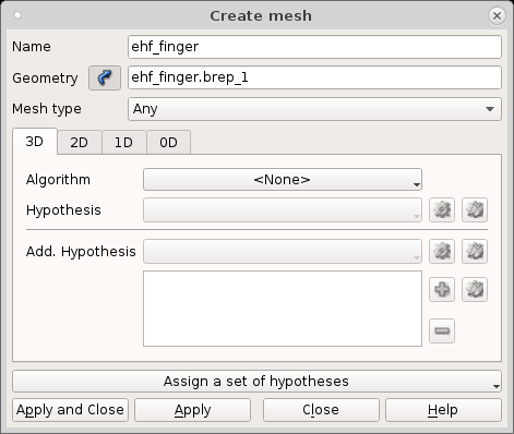
Fig. 3.38 To create new mesh, the user must first select the GEOM object in the Object Browser. Then one can define different types of meshes.

If the meshing computation was successful, the new mesh appeares in Object browser under the name that we specified in the dialog. See figure Fig. 3.39.

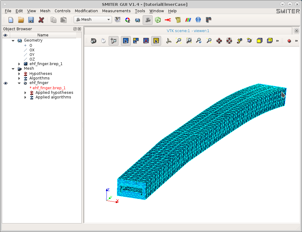
Fig. 3.39 Newly defined mesh is visible in the Object Browser, along with all other meshes.

Again we have to create groups that represent subsections for boundary conditions and material properties. To do that, right click on the mesh in the Object browser in the Mesh section and then Create Group. See figure Fig. 3.40.

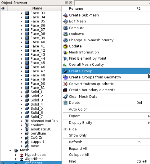
Fig. 3.40 To create group from mesh, right click on the object in the Object Browser and select Create Group.

New dialog appeares on the screen. First, the main mesh is selected. Then the user has to select the type of the element. Next the user can define the name of the mesh group. In the group type option one has to select Group on geometry. Then the user can navigate to the Object browser and select the group, defined in the Geometry section. The same name of the geometry group will appear in the Geometrical Object widget in the dialog Create Group. Then one has to click Apply. See figure Fig. 3.41.

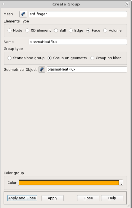
Fig. 3.41 To create group from mesh, select the type of geometrical entity that the new group will be constructed of. Then the user can create a standalone group, group on filter or group on geometry. To define groups from geometry, the user can select geometrical groups from Object Browser.

The new mesh group can be seen in the Mesh module. The user has to repeat those steps for every subsection. In the end all of the mesh groups can be seen in the Object browser. Refer to Fig. 3.42.

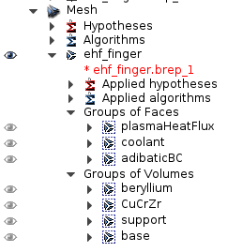
Fig. 3.42 All created meshes and thier groups can be visible in the Object Browser.

3.4.4. Defining The Model Properties

To move to ELMER module, select ELMER option from the menu. See figure Fig. 3.43.

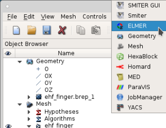
Fig. 3.43 Select ELMER option to move to Elmer module.

Then navigate to Elmer ‣ Case ‣ Create general case. The following dialog is displayed (figure Fig. 3.44).

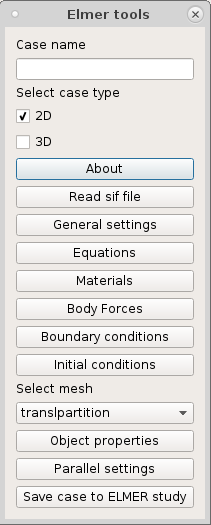
Fig. 3.44 In Elmer tools dialog the user can define basic setup for the Elmer case, such as boundaey conditions, material properties, etc.

3.4.4.1. Defining The Solver

Two main options from the main menu define the solver. First, user has to open General settings. Dialog appeares on the screen (figure Fig. 3.45).

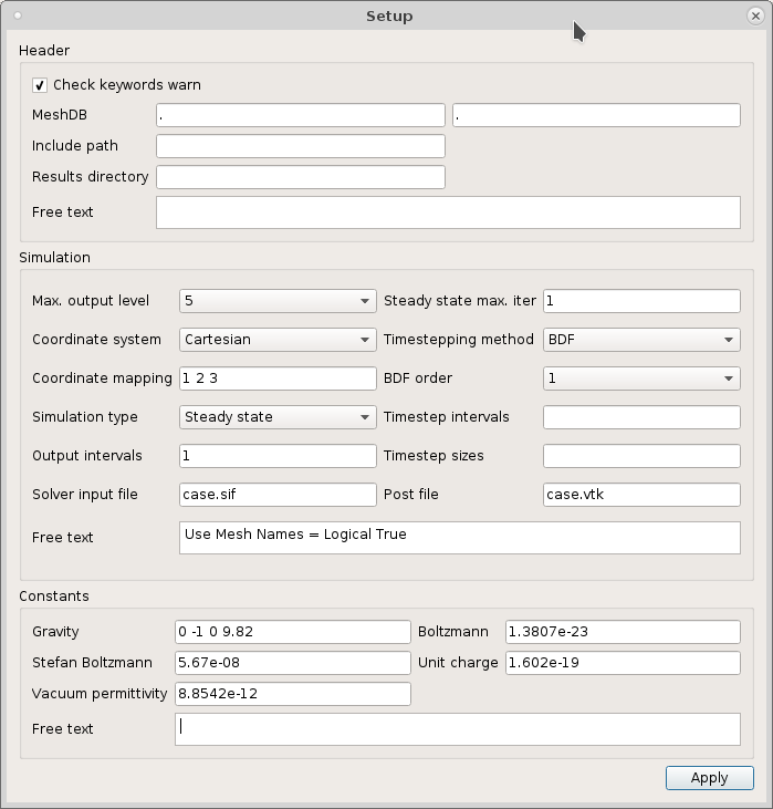
Fig. 3.45 For each case, the user can define different basic properties, such as simulation options, constants used in the case, results directory, etc.

In the dialog there are three sections (header, simulation and constants). In the header one can define the results directory. If left blank, the results are stored in the same folder as SIF file. Inthe simulation section different solver parameters can be defined. User should change the Post file to a file with VTK (.vtk) or VTU (.vtu) extension, instead of default (.ep) extension. In the constants segment the user can define different constants. In the end one has to click Apply to store changes.

Next step is to define the equation. To do that, click on Equations option in the main menu. See figure Fig. 3.46.

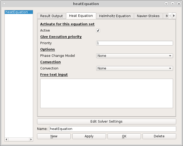
Fig. 3.46 Dialog to define equations used in the case. The user can define multiple equations if needed.

Here the user can define multiple different equations. In this tutorial heat equation is the only equation to choose. The user has to set equation to active. The execution priority is 1. With click on the Edit Solver Settings the user can define other properties. When the properties are applied, the user can click Apply. If another equation will be used in the case, click New, otherwise click OK.

3.4.4.2. Defining Material Properties

To determine material properties, click on Materials in the main dialog. New dialog appeares on the screen. See figure Fig. 3.47.

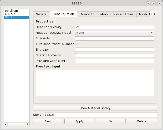
Fig. 3.47 Dialog to define material properties.

In this tutorial three materials with constant properties are defined.

	beryllium	CuCrZr	SS316
Density [ \(kg/m^2\) ]	1800	8800	7700
Heat Conductivity [ \(MW/m^2\) ]	150	330	20

Density is defined in General section and heat conductivity in Heat Equation section. To save changes, click Apply. To create new material, click New. When done, click OK.

3.4.4.3. Defining Boundary Conditions

To define boundary conditions, click on option Boundary conditions in the main menu. New dialog appeares on the screen. See figure Fig. 3.48.

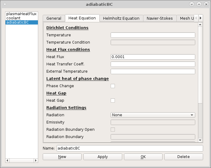
Fig. 3.48 Inside Elmer module the user can define different boundary conditions for different mathematical models, such as Heat equation, Helmholtz equation, Navier-Stokes equation, etc.

In this tutorial three boundary conditions with constant properties are defined.

• Plasma heat flux: \(q_{pl}=4.7 MW/m^2\)
• Heat transfer coefficient: \(T_{b}=80 C^{\circ}, HTC=13000 W/m^2\)
• Adiabatic boundary condition: \(q_{ad}=0 W/m^2\)

3.4.4.4. Assigning Properties To Sections

To assign material property to section, first select the mesh group, that represents a section that you want to assign the material to. Then click on Object properties in the main dialog. New dialog appeares on the screen. See figure Fig. 3.49.

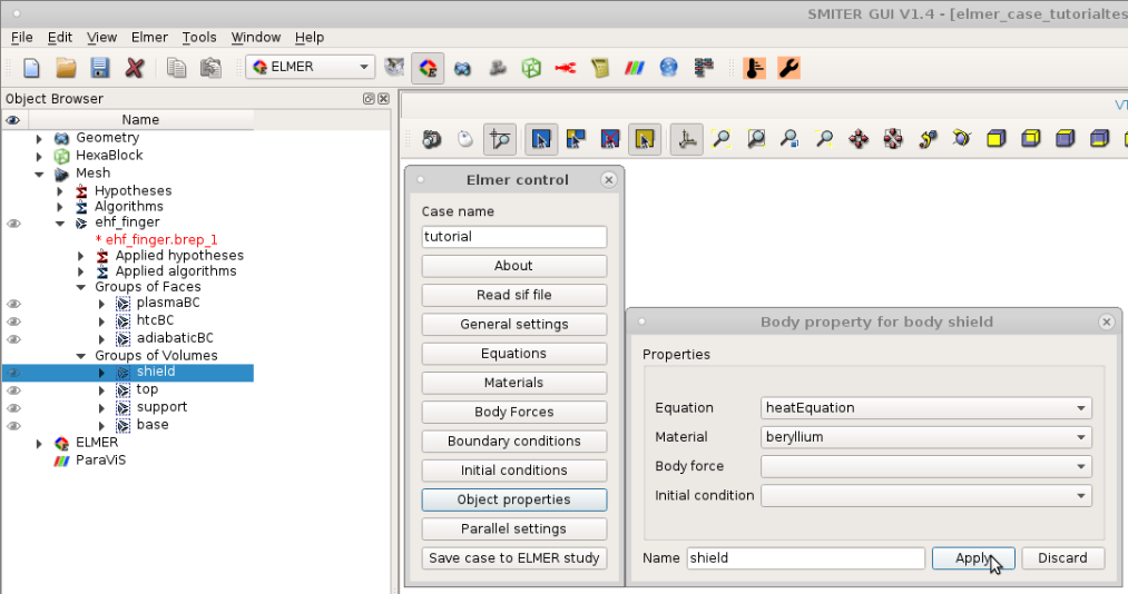
Fig. 3.49 To assign properties to sections, select group mesh in the Object Browser and then select material property.

The Body force and Initial condition are left blank. User has to define Equation and Material options according to the defined model. The same process is repeated for all the other materials and boundary conditions as well.

3.4.4.5. Store case to ELMER Study

After everything has been defined, one can store the case to study. To do that, click on option Save case to ELMER study. The dialog will close and new object with the name of the case will appear in the Object Browser under ELMER object. This new object contains ElmerGrid meshes and SIF file. If user right-clicks on it, four options appear on the screen. Refer to figure Fig. 3.50.

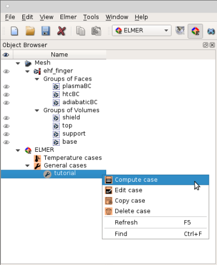
Fig. 3.50 By clicking on Compute case the computation starts. The output of the computation is stored to the folder specified in ELMER preferences, along with all the mesh and SIF files. With Edit case the user can edit and change the settings of the case. By clicking on Copy case the user can create new case, starting with the settings of the current case. Delete case option deletes the case from the current study.

3.4.4.6. Running the Computation

To run the computation, click on option Compute case. The computation runs. Navigate to the folder specified in the ELMER preferences. The following files are generated in the selected folder.

project
└── tutorial_map
   ├── ehf_finger.unv
   ├── mesh.boundary
   ├── mesh.header
   ├── mesh.names
   ├── mesh.nodes
   ├── mesh.elements
   ├── entities.sif
   ├── case.sif
   ├── case0001.vtu
   ├── case.log
   └── ElmerGrid.log

First the UNV was generated and then used to create ElmerGrid` files. Logfile ElmerGrid.log contains output information on mesh conversion from UNV to ElmerGrid. Then the command ElmerSolver was executed.

3.4.4.7. Viewing the result

New files are generated in the results folder.

• case0001.vtu: VTU results file with temperature data
• case.log: Log file with data on computation process.

The result of temperature distribution is shown in Fig. 3.51.

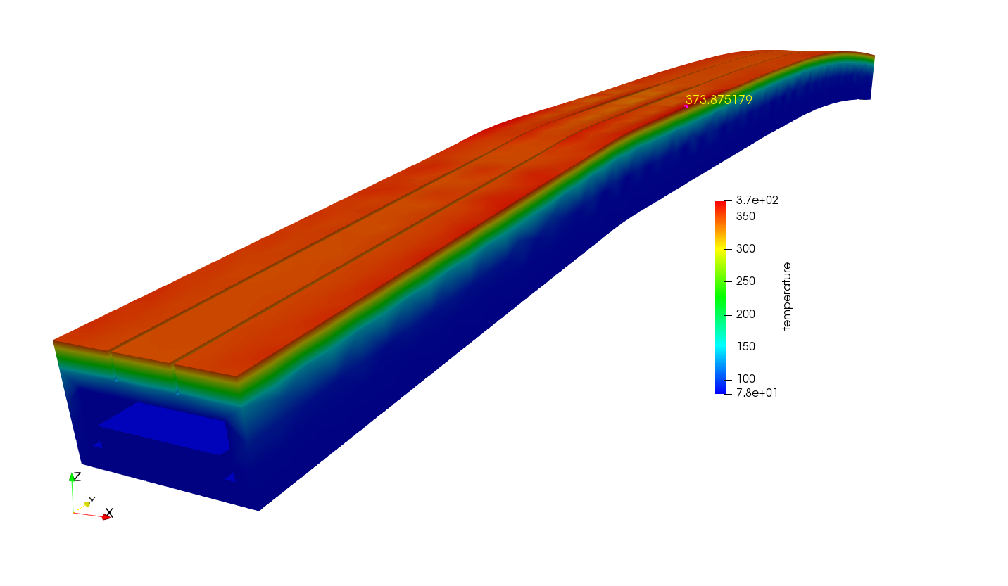
Fig. 3.51 Result of temperature distribution on EHF finger.