4.21. 3D Magnetic Field¶

Generally, in SMITER, the goal is to study field lines in axisymmetric magnetic field. For most cases, magnetic field is given in the form of equilibrium file with 2D data, that repeats itself on every step around the torus. The assumption of 3D field is different. In this case the magnetic field is represented as a 3D vector field, that contains magnetic field components in all three coordinate axes.

The purpose of taking into an account full 3D field is to study the effect of perturbations or anomalies of the magnetic field in the tokamak. Those perturbations could appear because of coil misalignment, deformation of the coil due to its mass, installation error of the coils, etc.

Full 3D field case inside SMITER was primarily designed for use on ITER tokamak geometry but can be easily extended to other tokamaks, as long as the input data follows a specified input format.

In this documentation, several studies on 3-D magnetic field are presented. These studies were performed in order to verify the accuracy of MAGTFM code.

First step: Create a uniform 3-D magnetic field and apply it to toroidal target of first wall panels (FWP) 4. The goal of this study was to verify the code by showing that for the axisymmetric 3-D magnetic field the result is the axisymmetric power deposition. One expects that the wetted area on every FWP 4 in toroidal direction should be the same.
Second step: Repeat the NF_55 benchmark case, but this time with 3-D magnetic field. First the study with axisymmetric magnetic case was prepared. One expects the same wetted area as per NF_55 benchmark case. Then the case was run with perturbed 3-D magnetic field. Results for both cases are presented here.
Third step: Use the full toroidal FWP 4 with circular plasma equilibrium. The goal was to again first use axisymmetric 3-D field and show that each panel has the same wetted area as one would expect. Then the perturbed 3-D magnetic field was studied. The differences in wetted area are presented here.
Fourth step: Take studies from step 3 and increase the helicity in order to magnify the differences in wetted areas. Both studies are presented in this chapter.

4.21.1. ENERGOPUL 3D field¶

This magnetic field represents the files produced inside the vacuum vessel by the nominal current flowing in the toroidal field (TF) coils. The number of nodes of the 3D structured grid, used for calculation of magnetic field was estimated for 1% accuracy in calculations of magnetic field using linear interpolation of the magnetic field between the mesh points.

Magnetic field is given in coordinate system $r, \varphi, z$. The plane $\varphi=0$ coincides with the plane $Y=0$ of Tokamak Global Coordinate System (TGCS), which also represents the midplane of TF coil number 1 (TFC-01 in Fig.[Fig. 4.76 ]). Positive direction of $\varphi$ corresponds to the anticlockwise direction, when viewed from above.

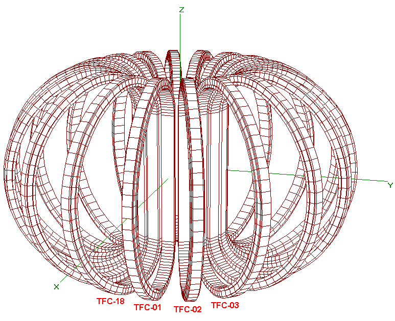
../../_images/magnetic_field_case_coils.png

Fig. 4.76 The model of toroidal field coils in the Tokamak Global Coordinate System. Note that the midplane of TF coil 1 coincides with $Y=0$ plane.

The whole 3D magnetic field data is divided in eighteen toroidal 20-degree segments. Notion “segment” is interpreted as the 20-degree toroidal sector taken from $-10^{\circ}$ to $10^{\circ}$ degree from the poloidal midplane of the corresponding magnetic coil. The following mesh was used for the representation of the field:

$3.7m \leq r \leq 8.7m$, step $\Delta r =0.1m$, 51 points in the radial direction.
$-5m \leq z \leq 5m$, step $\Delta z =0.1m$, 101 points in the vertical direction.
$\varphi$ at $20^{\circ}$ segment, step $\Delta \varphi = (20/29)$, 30 points in toroidal direction.

The number of all nodes for one segment is $51*101*30=154530$. The data is written with $R$ varying the fastest, then $Z$ and $\varphi$ varying the slowest.

String number	Content
1	$r_{1} \ \varphi_{1} \ z_{1} \ B_r \ B_{\varphi} \ B_z$
2	$r_{2} \ \varphi_{1} \ z_{1} \ B_r \ B_{\varphi} \ B_z$
…	…
51	$r_{51} \ \varphi_{1} \ z_{1} \ B_r \ B_{\varphi} \ B_z$
52	$r_{1} \ \varphi_{1} \ z_{2} \ B_r \ B_{\varphi} \ B_z$
…	…
102=5112	$r_{51} \ \varphi_{1} \ z_{2} \ B_r \ B_{\varphi} \ B_z$
103	$r_{1} \ \varphi_{1} \ z_{3} \ B_r \ B_{\varphi} \ B_z$
…	…
5151=511101	$r_{51} \ \varphi_{1} \ z_{101} \ B_r \ B_{\varphi} \ B_z$
5152	$r_{1} \ \varphi_{2} \ z_{1} \ B_r \ B_{\varphi} \ B_z$
5153	$r_{2} \ \varphi_{2} \ z_{1} \ B_r B_{\varphi} \ B_z$
…	…
154530=5130101	$r_{51} \varphi_{30} \ z_{101} \ B_r \ B_{\varphi} \ B_z$

As seen each line contains six values separated by spacebars:: three coordinates ($r, \ \varphi, \ z$) and three field components ($B_r, \ B_{\varphi}, \ B_z$). The current assumed in each coils is $I_0=-9.128MA$, which produces at the radius $6.2m$ the nominal value of magnetic field $-5.3T$.

4.21.1.1. Ideal ENERGOPUL field¶

Ideal field from ENERGOPUL is give just for one segment, since one assumes that the field is axisymmetric for each coil and no coils are misaligned, thus no perturbation appears in the field. The database of the magnetic field produced by the TF coils with the nominal current in the segment #1 is stored in the IDM system in ZIP file with the number 47UQUV or in the examples/magtfm folder of SMITER directory with the name T_47UQUV_v1_3. The IDM folder can be found using the link 47UQUV.

4.21.1.2. ENERGOPUL field with perturbations¶

Deviation of the TF coil current centrelines (CCLs) from their ideal position and shape leads to the 3D perturbation of the toroidal magnetic field. In this specific example, ripple in the 3D field is caused by type “V3” misalignment of the TF coil CCLs distorted by EM loads, assuming the nominal value and direction of current in each coil. Magnetic field produced by the TF coils with misalignments of the coil CCLs “V3” ($B_r, \ B_{\varphi}, \ B_z$) can be calculated as a superposition of the magnetic field from the ideal TF coils ($B_{r0}, \ B_{\varphi 0}, \ B_{z0}$), which is given in the database of the ideal ENERGOPUL field given with reference number 47UQUV and the magnetic field ($\Delta B_{r}, \ \Delta B_{\varphi}, \ \Delta B_{z}$) given in ZIP file with reference number Y2KYAD or in the examples/magtfm folder of SMITER directory with the name V3_Y2KYAD.

Navigate to examples/magtfm and run the python script superposition.py. New folder superposition will be created that will contain 18 files with 3D magnetic field inside.

4.21.2. SMITER 3D file format¶

Input file to SMITER with 3D magnetic field has the following format:

Zeta grid
Nzeta
  Zeta_1
  Zeta_2
  :
  Zeta_Nzeta

R grid
Nr
  R_1
  R-2
  :
  R_Nr

Z grid
Nz
  Z_1
  Z_2
  :
  Z_Nz

B(component:{x,y,z},zeta,r,z). Toroidal sector in negative y adjoining x=0.
Bx(R_1, Z_1, Zeta_1) By(R_1, Z_1, Zeta_1) Bz(R_1, Z_1, Zeta_1)
:
Bx(R_1, Z_1, Zeta_Nzeta) By(R_1, Z_1, Zeta_Nzeta) Bz(R_1, Z_1, Zeta_Nzeta)
Bx(R_2, Z_1, Zeta_1) By(R_2, Z_1, Zeta_1) Bz(R_2, Z_1, Zeta_1)
:
Bx(R_Nr, Z_1, Zeta_Nzeta) By(R_Nr, Z_1, Zeta_Nzeta) Bz(R_Nr, Z_1, Zeta_Nzeta)
Bx(R_1, Z_2, Zeta_1) By(R_1, Z_2, Zeta_1) Bz(R_1, Z_2, Zeta_1)
:
Bx(R_Nr, Z_Nz, Zeta_Nzeta) By(R_Nr, Z_Nz, Zeta_Nzeta) Bz(R_Nr, Z_Nz, Zeta_Nzeta)

The magnetic field is given in structured grid with equally spaced steps in each direction ($\zeta, R, Z$). First, one set of sample points is given as specified above. $R$ and $Z$ are specified in metres, while $\zeta$ is specified in radians, one value per line. Magnetic field $B$ is given in Cartesian components, one vector per line ($Bx, By, Bz$). Note that for SMITER input, the B vectors are ordered with $\zeta$ varying the fastest, then $R$ and finally $Z$ varying the slowest. Each of the 4 items ($\zeta$, $R$, $Z$ and $B$ ) in the file is separated from the next by a blank line, each item starts with a description line, followed by the array size, except in the case of B.

../../_images/magnetic_field_cs_energopul_vs_smiter.svg

Fig. 4.77 The data provided by ENERGOPUL specifies the magnetic components given in cylindrical polar angle $\varphi$, which is measured clockwise about the vertical $Z$ axis, viewed from above (left). On the other hand, SMITER works with the polar angle $\zeta$, which is measured anticlockwise about the vertical $Z$ axis (right). For both of those systems, the origin $\varphi=\zeta=0$ corresponds to the positive $X$ - axis. If data is given in $\varphi$, both coordinates and vectors should be converted to correspond to $\zeta$.

To convert the superposition ENERGOPUL files into MAGTFM file format with 577 steps in toroidal $\zeta$ direction run the python3 script get_full_superposition_field.py. File full_superposition_field.txt will be created and can be imported to SMITER study as MAGTFM file. The file

Note

It is again important to note the difference between coordinate systems used in the SMITER 3D field computation. The data provided by ENERGOPUL specifies the magnetic components given in cylindrical polar angle $\varphi$, which is measured clockwise about the vertical $Z$ axis, viewed from above. On the other hand, SMITER works with the polar angle $\zeta$, which is measured anticlockwise about the vertical $Z$ axis. For both of those systems, the origin $\varphi=\zeta=0$ corresponds to the positive $X$ - axis. See Fig. 4.77.

4.21.3. Inputs and Outputs¶

The input parameters that correspond to 3D magnetic field case, are

data_layout: Parameter data_layout corresponds to the format of input file that contains 3D magnetic field components, given in .txt file. For working with full $360^{\circ}$ ITER magnetic field, there are two main options that should be used in this case.
- data_layout=14: Option 14 corresponds to magnetic field data, where the number of points in toroidal direction ($\zeta$ direction) $n_{\zeta}$ subtracted by 1 ($n_{\zeta}-1$) is a prime number. This is unfortunate because of the existing Fourier transform algorithm then equires an expensime matrix multiply, that is possibly also subject to significant rounding error.
- data_layout=12: This option corresponds to the magnetic field data where the number of points in toroidal direction ($\zeta$ direction) $n_{\zeta}$ subtracted by 1 ($n_{\zeta}-1$) is not a prime number. If possible, this option should be used instead of option 14.
zeta_start: Toroidal angle $\zeta_{start}$ of first point in samples (degrees). This is the angle of the beginning of the first point in the first segment, in case of ENERGOPUL data this parameter should be set to $-10^{\circ}$.
plot_bcartx: Plot option that creates 3D vtk plot of magnetic field components B. The magnetic field can be thus visualized in Paraview.
i_requested: This number is the product of toroidel magnetic field $B_T$ at the nominal radial position $R$, i.e. i_requested= $B_TR$.
mode_cutoff: Relative mode cut-off amplitude, default $.0001$.

4.21.3.1. ITER Case with uniform 3D magnetic field¶

In this section case with uniform 3D toroidal field will be presented. This magnetic field has no perturbations and is constant in $\varphi$ direction, so we expect the same power deposition on every panel in toroidal direction.

The case is stored in trid_skel_uniform_field.hdf in ~/smiter/salome/magtfm/ folder. Open the study and move to Mesh module

target: Full toroidal target with FWP 4. Target was generated from single panel fw4t.vtk, located in smiter-aux repository and used in test case Val-F11-fw264t-fw4t.
shadow: Full toroidal shadow of panels 2, 3, 4, 5 and 6. Shadow was made by copying the target and using translation and rotation functions in Mesh module. Distance in z-direction between panels is 12 mm.

Now move to SMITER module and examine the equilibrium file (53.eqdsk). The LCFS and Limiter contour can be seen in Fig. 4.78. This is an equilibrium with circular LCFS and was moved aditionally in r-direction (beq_rmove) by $-20mm$ and in z-direction (beq_zmove) by $1090mm$ to face the target.

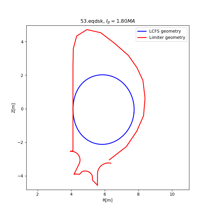
../../_images/magnetic_field_case_53eqdsk.png

Fig. 4.78 The LCFS and Limiter contour of equilibrium file.

Full 3D magnetic field can be seen in Fig. 4.79.

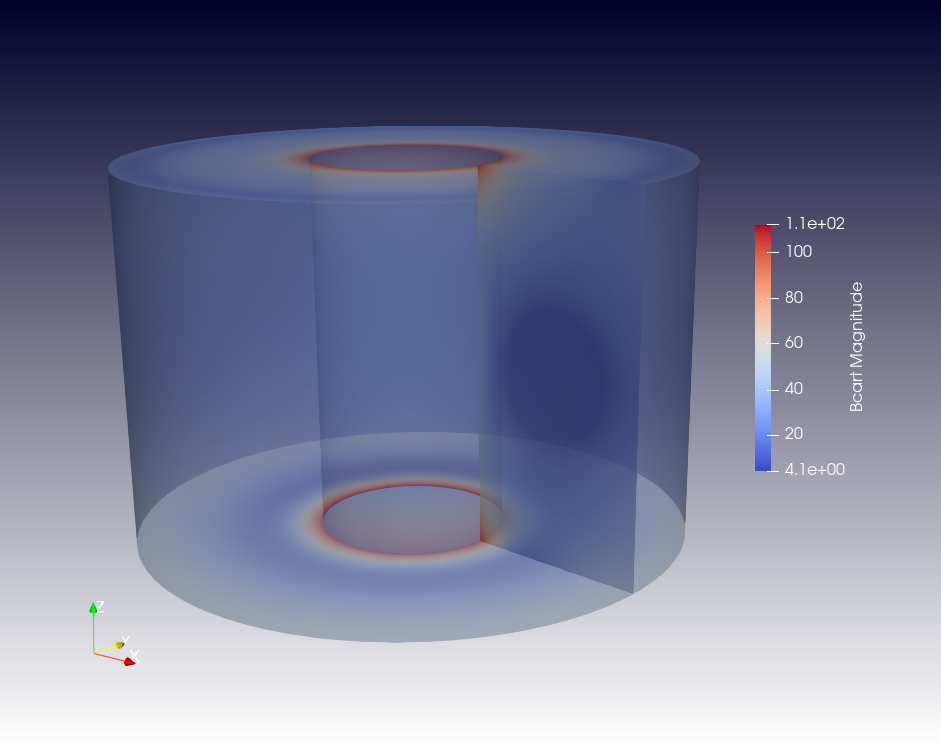
../../_images/magnetic_field_case_3Duniform_field.png

Fig. 4.79 Magnitude values of uniform magnetic field.

Power deposition is calculated with double exponential formula and input data is as follows:

Power loss $P$ = 5 MW
Decay length $\lambda$ = 37 mm
Decay length near $\lambda$ = 3 mm

New inputs for MAGTFM code are as follows:

Data layout data_layout = 12
Plot of B-field plot_bcartx = .true.

Option plot_bcartx controls production of .txt file only if mag_output_file='null'. There is no additional parameter for powcal, it simply recognises that and input 3D field file with suffix .txt contains an fmesh object. This object comes with trilinear interpolation to return magnetic field values at a given point within their domain of definition.

The result can be seen in [ Fig. 4.80 ]

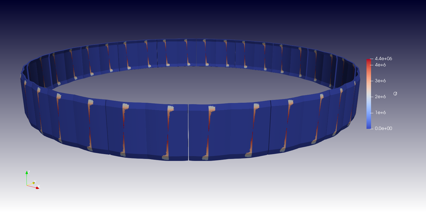
../../_images/magnetic_field_case_3Duniform_field_result.png

Fig. 4.80 Result of first wall panel 4 in toroidal direction using the uniform 3D magnetic field.

The goal of this study was to verify the code by showing that for the axisymmetric 3-D magnetic field the result is the axisymmetric power deposition. One expects that the wetted area on every FWP 4 in toroidal direction should be the same.

The result is shown in Fig. 4.80. The pattern is the same in every panel, which corresponds to uniform 3D field.

4.21.3.2. ITER NF55 Case with 3D magnetic field¶

Two studies will be presented in this case. The first one contains magnetic field with no perturbations and is constant in $\varphi$ direction, so we expect the same power deposition on every panel in toroidal direction. The second one contains 3-D perturbed magnetic field. The difference in this case is that magnetic field components $B_{r}$ and $B_{z}$ are not equal to 0.

4.21.3.2.1. Uniform Field¶

The case is stored in nf_55_03319_2015_with_magtfm.hdf in ~/smiter/salome/magtfm/ folder. Shadow and target are shown in Fig. 4.81. Open the study and move to Mesh module. The meshes are generated from the newest CAD model as follows

shadow_CAD_align: nf55 shadow where the target panel is aligned with other panels.
shadow_CAD: nf55 shadow where the shadow panels are moved outward the plasma by 5 mm as in the benchmark case.
CAD_FWP4_minus25_mesh: nf55 target that is moved backwards by 25 mm and is thus aligned with the shadow.
CAD_FWP4_minus20_mesh: nf55 target that is moved backwards by 20 mm so that it is at the original position as the benchmark version of the target.

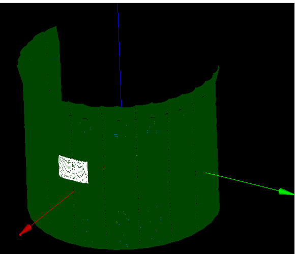
../../_images/magnetic_field_shadow_target_nf55.svg

Fig. 4.81 Shadow (green) and target (white) of nf_55 axisymmetric 3-D magnetic field.

Result is shown in Fig. 4.82.

../../_images/magnetic_field_nf_vs_nf_axisymmetric.svg

Fig. 4.82 Comparison of the NF_55 benchmark result (left) and FWP4 using the uniform 3D magnetic field. One can see that the results are similar.

4.21.3.2.2. Non Uniform Field¶

The case is stored in nf_55_03319_2015_with_magtfm_perturbation.hdf in ~/smiter/salome/magtfm/ folder. Results are shown in Fig. 4.83.

../../_images/benchmark_magtfm_perturbation_vs_axisymm_result.svg

Fig. 4.83 Result of nf55 case with 3-D magnetic perturbed field. One can see that the peak power deposition and wetted area are slightly different than in axisymmetric 3-D magnetic field case.

4.21.3.2.2.1. Full 3-D Magnetic Field¶

In the figure Fig. 4.84 the 3-D magnetic field in full toroidal direction is shown. This field was generated from the energopul files and converted into appropriate MAG format. To obtain the MAG format, run the get_full_superposition_field.py as explained in the $SMITER_EXAMPLES_DIR/README.rst directory. The output of the script is a file named full_superposition_field.txt in MAG format.

../../_images/3D_full_magnetic_field.png

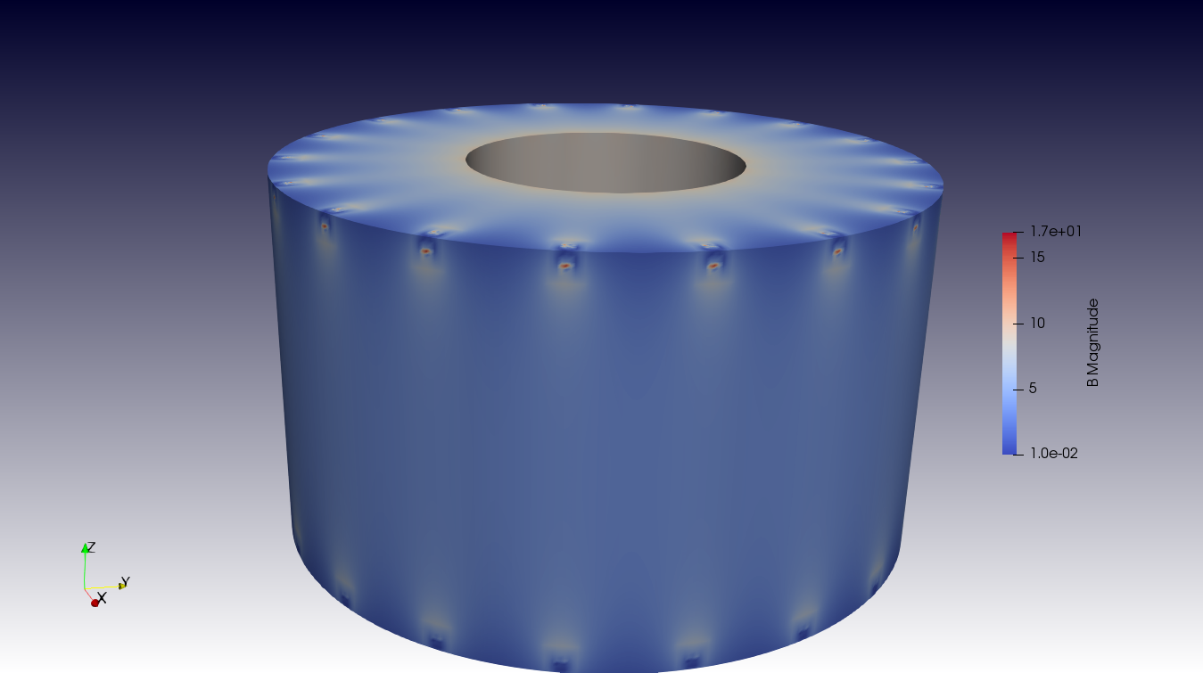
Fig. 4.84 3D magnetic field produced from energopul data.

Figure Fig. 4.85 has two plots that show the change of magnetic components ($B_x$, $B_y$ and $B_z$) in toroidal direction at $R=4.03m$ and $Z=1.01m$. The first plot shows the change of $B_z$ and the second one shows the change of $B_x$ and $B_y$.

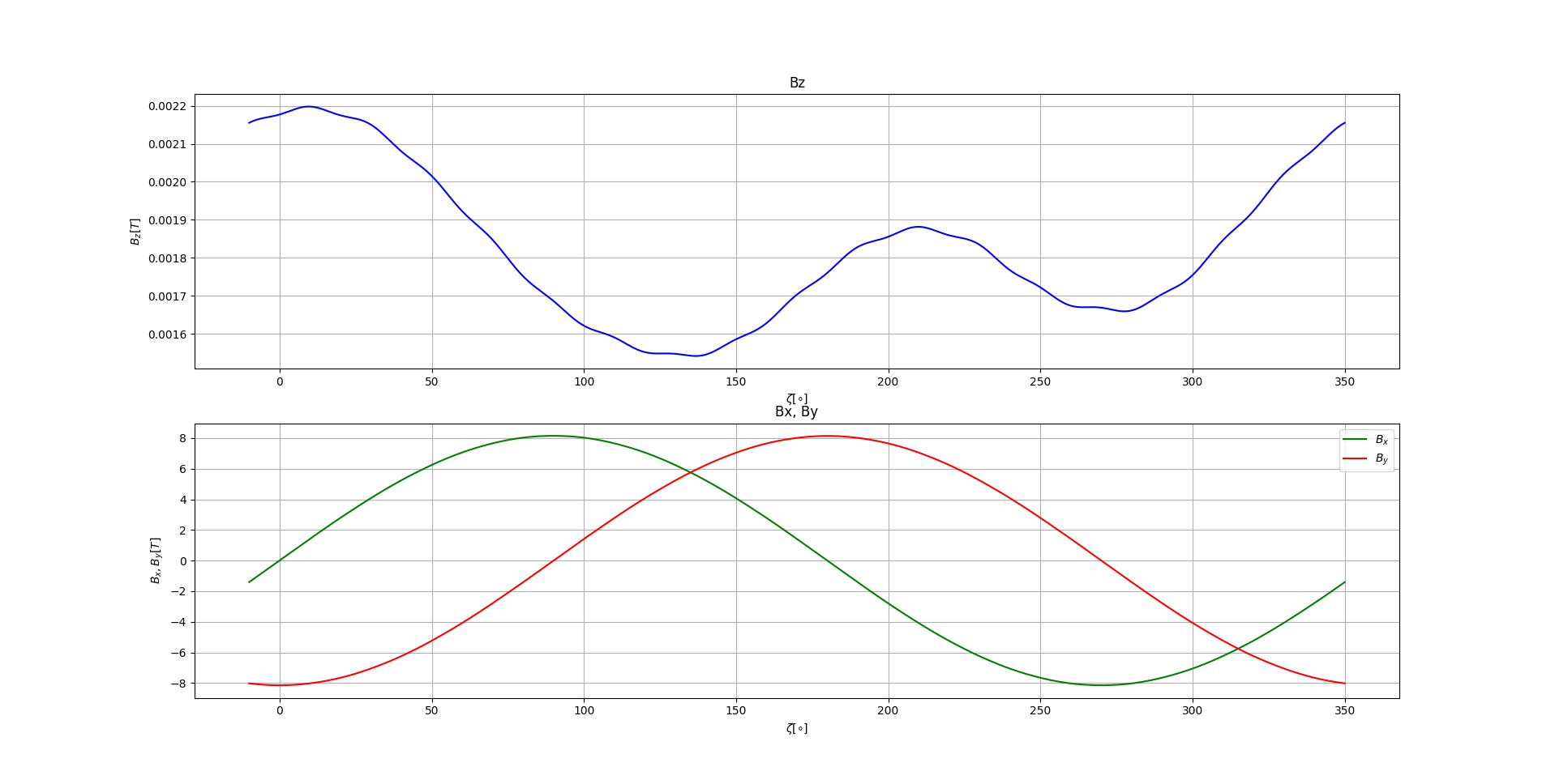
../../_images/3D_full_magnetic_field_components.png

Fig. 4.85 3D magnetic field components changing in toroidal direction.

4.21.3.2.2.2. Comparison of Uniform 3D Field with Non Uniform 3D Field¶

The goal of this comparison is to show differences between uniform and non uniform case and to find out which panels will get more power deposition. Two studies, one with uniform field and other with non uniform field, are as follows:

Uniform_CAD_target.hdf
Non_Uniform_CAD_target.hdf

The positions of individual panels in full toroidal target are shown in Fig. 4.86.

../../_images/magnetic_field_panels_position_colors.svg

Fig. 4.86 3D magnetic field components changing in toroidal direction.

4.21.3.2.3. Uniform Field¶

To open study with uniform 3D magnetic field, navigate to study/magtfm and open file Uniform_CAD_target.hdf. The input files are a follows:

target: Contains Uniform_CAD_target, which is built of eighteen first wall panels 4 in toroidal direction.
shadow: 18 first wall panels (ID = 1, 2, 3, 4, 5 and 6) in toroidal direction. See Fig. 4.87.
equilibrium file: 53.eqdsk. Circular plasma, moved in $R$ and $Z$ to the contact point with FWP 4. The LCFS and Limiter contour can be seen in Fig. 4.78.
MAG file: MAGTFM_Zeta_coor_577_Pure_toroidal.txt. Magnetic field file with zero values in $R$ and $Z$ direction. It contains 577 steps in $\zeta$ direction.

../../_images/magnetic_field_case_uniform_CAD_shadow_target.svg

Fig. 4.87 Target and shadow of case with uniform 3D magnetic field.

Difference in power deposition was studied for every panel across toroidal cross-section for three different z positions. In Fig. 4.81 one can see three different cross sections, taken at $z=700mm$, $z=1000mm$ and $z=1320mm$.

../../_images/magnetic_field_uniform_CAD_target_axes.svg

Fig. 4.88 Positions of cross-sections used to compare power deposition of each individual panel.

To get power deposition at the specific height ( $z$ ) for each panel, select the vtk file in Pipeline Browser and click apply ( green button in Properties tab, as shown in Fig. 4.89.

../../_images/magnetic_field_apply_properties.svg

Fig. 4.89 Pipeline Browser with Properties tab. Click Apply to activate vtk object.

Then move to File ‣ Save Data… and type Cell Data to Point Data and hit Enter. New object will appear in the Pipeline Browser. See Fig. 4.90. After selecting the new object CellDataToPointData1 one can observe different properties on this object. The power deposition Q is now defined on nodes. See Properties tab and ParaView documentation for more details on interpolation.

../../_images/magnetic_field_cell_data_to_point_data.svg

Fig. 4.90 Object CellDataToPointData1 has values specified on nodes, unlike uniform_CAD_target.vtk, that has data on cells.

Again select CellDataToPointData1 object and click Apply in the Properties tab. Then again move to Filters ‣ Search and type Plot On Intersection Curves and hit Enter. In Fig. 4.92 one can see that new object appeared in Pipeline Browser. Next step is to define the intersection plane. In the Properties tab move to Plane Parameters section, set Origin to $x=0$, $y=0$ in $z=700$ and Normal to $n_x=0$, $n_y=0$ in $n_z=1$, as shown in Fig. 4.92. Cross-section plane with the panels is shown in Fig. 4.91.

../../_images/magnetic_field_plane_vs_panels.svg

Fig. 4.91 Intersection plane with FWPs 4.

Origin defines the point on the plane and normal defines the orientation of the plane. Then click Apply in the properties tab. New curves are generated at the intersection of the CellDataToPointData1 object and the plane specified in Properties tab of PlotOnIntersectionCurves1 object. See Fig. 4.92.

../../_images/magnetic_field_plot_on_intersection_curves.svg

Fig. 4.92 Intersection curves of SMITER result and intersecting plane.

To export curve data, select the object in Pipeline Browser and go to Filters ‣ Search…. Each individual curve and its data will then be stored in a .csv file.

Power deposition on every panel in $\zeta$ direction is shown in Fig. 4.93 for $z=700mm$.

../../_images/magnetic_field_uniform_CAD_target_z700.svg

Fig. 4.93 Power deposition around the torus for FWP 4 (left) and power depositions for individual panels, compared with each other (right) for $z=700mm$. One can see that pattern is the same round the torus and there is almost no differences in power deposition between panels.

4.21.3.2.4. Non Uniform Field¶

To open study with non uniform 3D magnetic field, navigate to study/magtfm and open file Non_Uniform_CAD_target.hdf. The input files are similar to the uniform study, the difference is in MAG file, which is in this case MAGTFM_Zeta_coor_577, which is 3D magnetic field with perturbation, as discussed in ENERGOPUL field with perturbations section. Note that this field contains 577 steps in $\zeta$ direction as well.

Power deposition on every panel in $\zeta$ direction is shown in Fig. 4.94 for $z=700mm$.

../../_images/magnetic_field_non_uniform_CAD_target_z700.svg

Fig. 4.94 Power deposition around the torus for FWP 4 (left) and power depositions for individual panels, compared with each other (right) for $z=700mm$. In this case one can see differences in power deposition between individual panels.

4.21.3.2.5. Uniform Field - Helicity¶

This study can be found in study/magtfm/Uniform_CAD_target_helicity.hdf. The difference between this study and Uniform_CAD_target.hdf is different helicity, that can be changed with MAGTFM parameter i_requested. Power deposition on every panel in $\zeta$ direction is shown in Fig. 4.95 for $z=700mm$.

../../_images/magnetic_field_uniform_CAD_target_helicity_z700.svg

Fig. 4.95 Power deposition around the torus for FWP 4 (left) and power depositions for individual panels, compared with each other (right) for $z=700mm$ for uniform field with increased helicity. One can see that the wetted area has increased in toroidal direction.

4.21.3.2.6. Non Uniform Field - Helicity¶

To open study with non uniform 3D magnetic field, navigate to study/magtfm and open file Non_Uniform_CAD_target_helicity.hdf. The difference between this study and Non_Uniform_CAD_target.hdf is different helicity, that can be changed with MAGTFM parameter i_requested.

Power deposition on every panel in $\zeta$ direction is shown in Fig. 4.96 for $z=700mm$.

../../_images/magnetic_field_non_uniform_CAD_target_helicity_z700.svg

Fig. 4.96 Power deposition around the torus for FWP 4 (left) and power depositions for individual panels, compared with each other (right) for $z=700mm$ for non uniform 3-D magnetic field with increased helicity. There are differences in wetted areas and peak power depositions in individual panels.

4.21.3.2.7. Comparison of Power Deposition¶

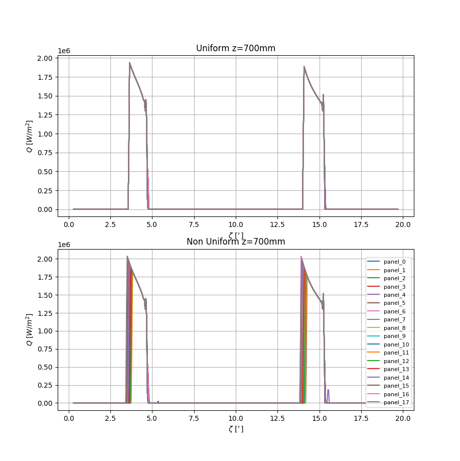
../../_images/magnetic_field_uniform_nonuniform_fixed.png

Fig. 4.97 Comparison of power deposition of all panels in toroidal direction for different configurations.

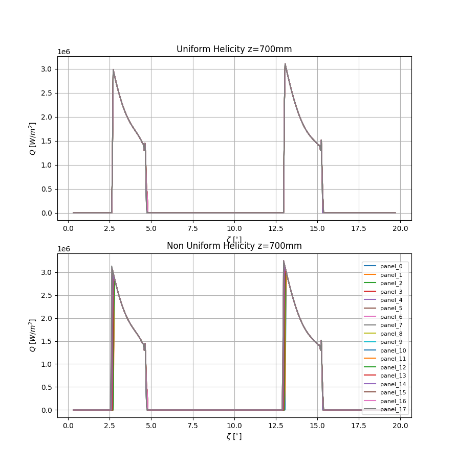
../../_images/magnetic_field_uniform_nonuniform_helicity_fixed.png

Fig. 4.98 Comparison of power deposition of all panels in toroidal direction for different configurations.

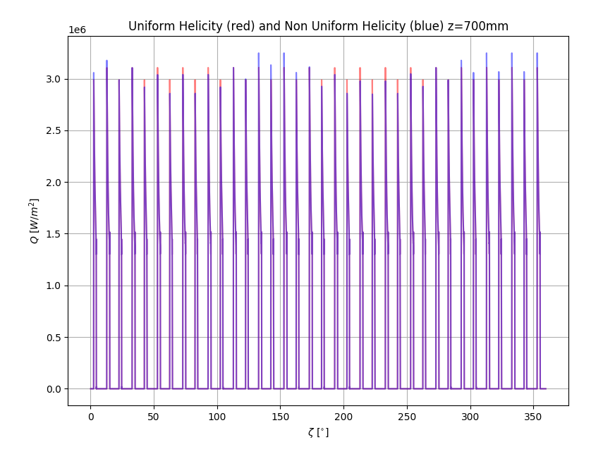
../../_images/magnetic_field_uniform_nonuniform_helicity_all.png

Fig. 4.99 Comparison of power deposition of all panels in toroidal direction for different configurations.

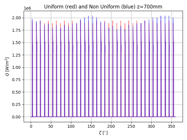
../../_images/magnetic_field_uniform_nonuniform_all.png

Fig. 4.100 Comparison of power deposition of all panels in toroidal direction for different configurations.

../../_images/magnetic_field_uniform_CAD_target_z700_q_vs_zbdotn.svg

Fig. 4.101 Comparison of power deposition of all panels in toroidal direction with $B . n$ distribution.

../../_images/magnetic_field_non_uniform_psista_all_vs_ind.svg

Fig. 4.102 Power deposition of all panels in toroidal direction (left) and power deposition of all panels moved to the position of first panel (between $0^{\circ}$ and $20^{\circ}$).