4.15. SMITER-PFCFLUX benchmark ‘HNB FW study’ Test case
4.15.1. Introduction
The purpose of the HNB FW study was to measure
the worst case heat loads on FW panels 14NE and 15NE, located around
the HNB-DNB
ports.
The scenario is an outer limiter configuration, operated at half-field (2.65T)
and I_p=5MA with an assumed P_sol=5MW with the longest possible decay length
of 29 millimeters. The EQDSK file is glimOWL175cm5p0MA2p65T_t10s_RDMR.txt.
This report examined the 14NE and 15NE panels and evaluate the worst
case heat loads in the case of a outer limiter configuration. The misalignment
of the shadow panels is also considered and the results mainly focus on results
of the case with the highest resolution target mesh and the misaligned shadow
mesh.
To further see how vertical shifts affect the panels, the EQDSK is vertically shifted from 500 mm to -500 mm with 100 mm increments.
Since the software is still in development along the version release number the GIT hash string is also provided.
The version of SMITER used:
SMITER release/1.6: 9dba7d9aa03e7f1498cc48a5b7615b4656550040
The field line ray trace program SMARDDA version:
smardda_lib: 7cef21bff13f1ff8ae10ebbfcd871a0af4319202smardda_pfc: 3db912ffb0425ee9614f5a4738f188703ccd8dfe
4.15.2. Input data
4.15.2.1. Meshes
Target mesh consists of panels 14NE and 15NE. There are three variants of the mesh:
- Low resolution variant with maximum 10 mm triangle edge length
- Higher resolution variant with maximum 5 mm triangle edge length
- Same as second but with refined panel edges that contain triangles with maximum 1 mm triangle edge length
Note
The low and higher resolution both have holes, while the refined mesh is without holes
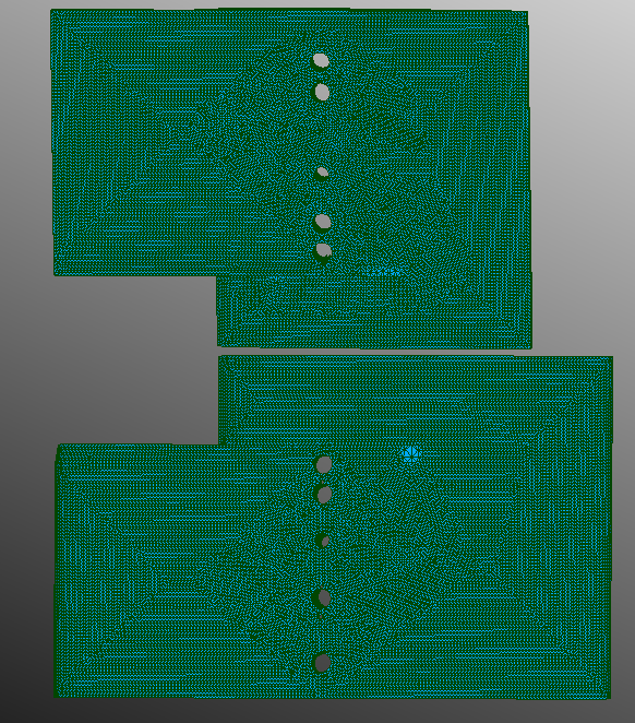
Fig. 4.36 Mesh 14NE15NE with maximum triangle edge length 10 mm
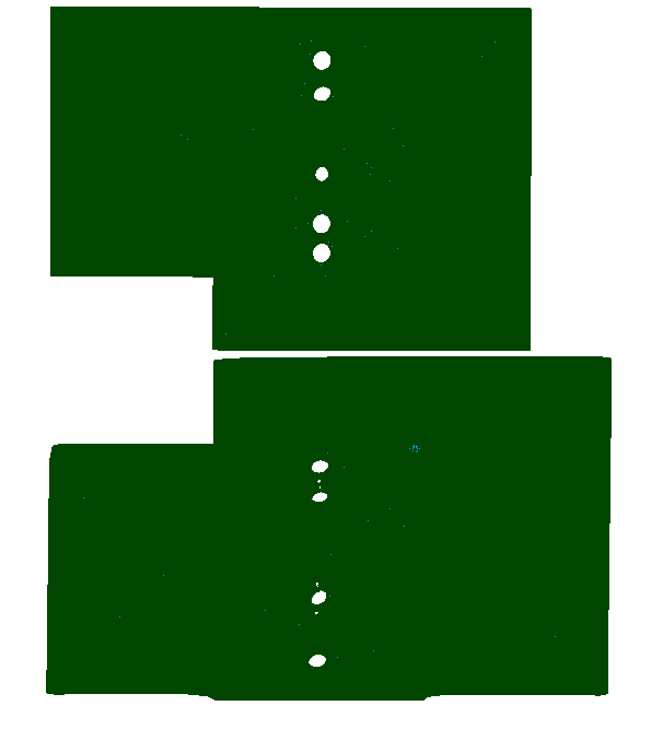
Fig. 4.37 Mesh 14NE15NE with maximum triangle edge length 5 mm
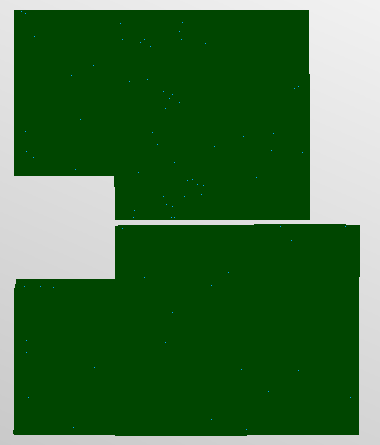
Fig. 4.38 Mesh 14NE15NE with maximum triangle edge length 5 mm with refined panel edges that contain triangles with maximum triangle edge length 1 mm
Differences between the meshes:
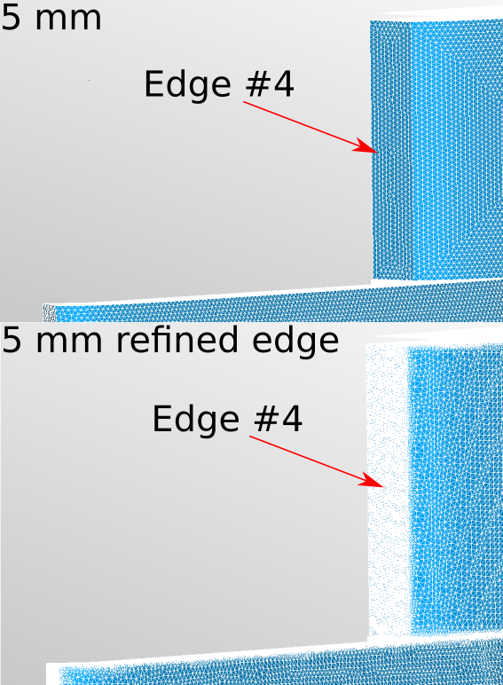
Fig. 4.39 Comparison of panel edges for 5 mm and 5 mm + refined 1 mm
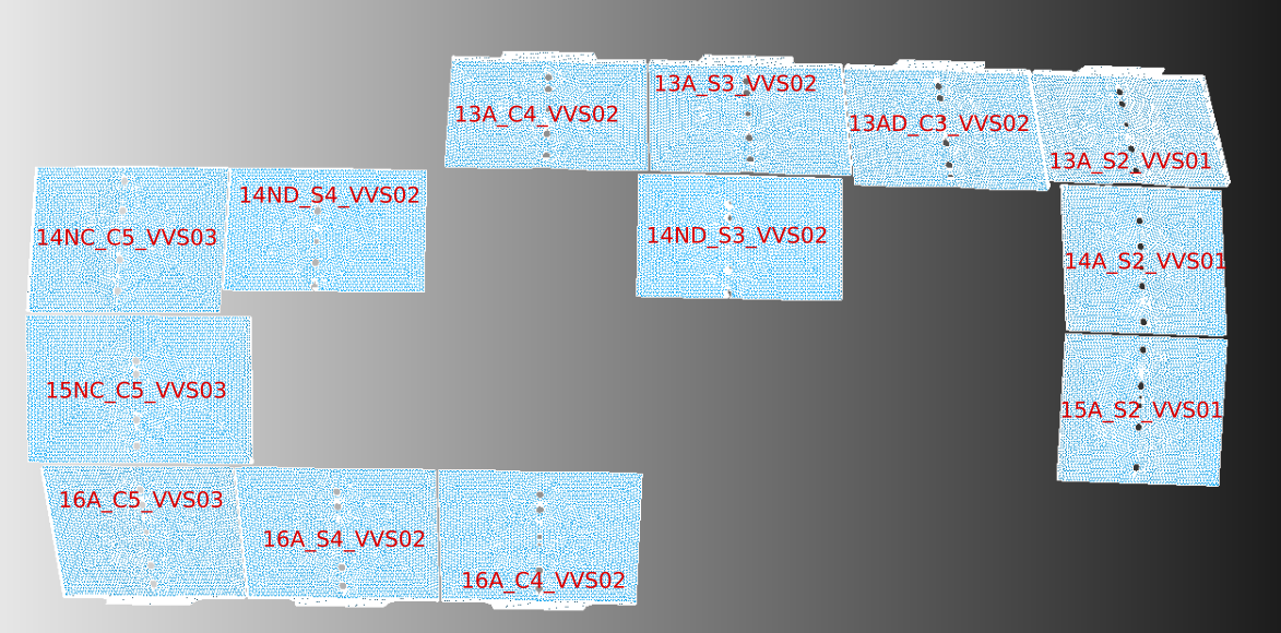
For shadowing the following list of meshes were used. All were meshed with maximum triangle edge length 25 mm:
- 13A_S2_VVS01
- 13A_S3_VVS02
- 13A_C4_VVS02
- 14A_S2_VVS01
- 13AD_C3_VVS02
- 14NC_C5_VVS03
- 14ND_S3_VVS02
- 14ND_S4_VVS02
- 15A_S2_VVS01
- 15NC_C5_VVS03
- 16A_S4_VVS02
- 16A_C5_VVS03
- 16A_C4_VVS02
Note
Shadowing meshes are translated to allow for worst case misalignments between neighboring panels. Translations are done parallel to the insertion/installation axis of each shadow FW panels.
The following table shows the translation vector for each shadow panel. Namely, the translation is done by 5 mm in the direction of insertion/installation of each panel respectively.
All values are in millimeters and values are rounded to the second digit.
| Panel | dx | dy | dz |
|---|---|---|---|
| 13A_S2_VVS01 | 3.44 | 2.9 | 2.1 |
| 13A_S3_VVS02 | 2.25 | 3.9 | 2.1 |
| 13A_C4_VVS02 | 1.55 | 4.25 | 2.1 |
| 14A_S2_VVS01 | 3.8 | 3.2 | 0.6 |
| 13AD_C3_VVS02 | 2.9 | 3.44 | 2.1 |
| 14NC_C5_VVS03 | 0.0 | 4.95 | 0.6 |
| 14ND_S3_VVS02 | 0.85 | 4.9 | 0.6 |
| 14ND_S4_VVS02 | 0.85 | 4.9 | 0.6 |
| 15A_S2_VVS01 | 3.2 | 3.2 | -0.4 |
| 15NC_C5_VVS03 | 0.0 | 4.95 | 0.6 |
| 16A_S4_VVS02 | 0.8 | 4.5 | -2.0 |
| 16A_C5_VVS03 | 0.8 | 4.5 | -2.0 |
| 16A_C4_VVS02 | 1.55 | 4.3 | -2.0 |
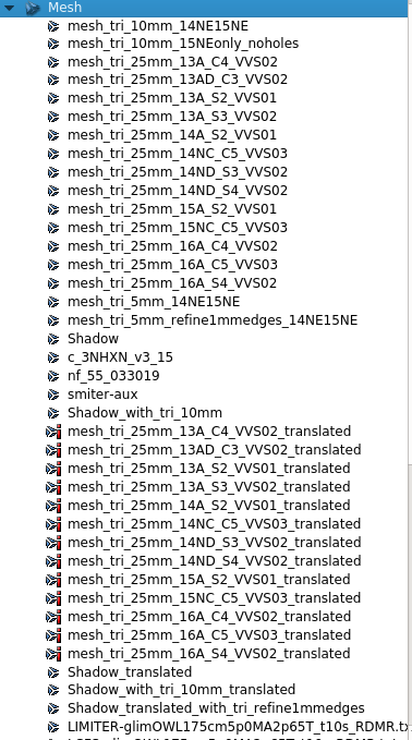
The translated shadow meshes in the HNB.hdf carry the name of the mesh and the
suffix _translated.
The change is not visible from a plane, but it impacts the results significantly since the wetted on the shadowed or target mesh depends on the surrounding meshes.
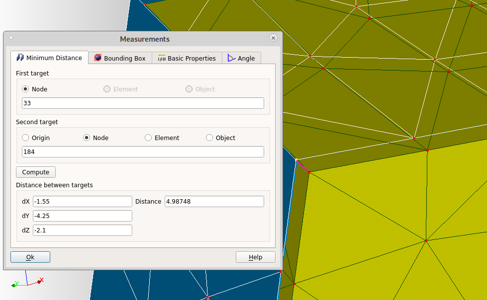
Fig. 4.40 Display of the translation on mesh of panel 13A_C4_VVS02
4.15.2.2. Equilibrium
The equilibrium used is EQDSK-G glimOWL175cm5p0MA2p65T_t10s_RDMR.txt.
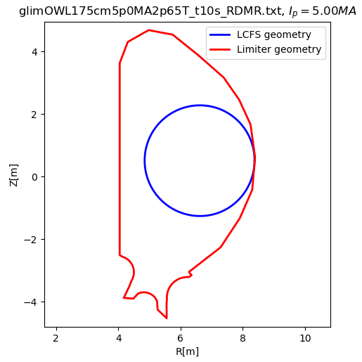
Fig. 4.41 Written limiter and plasma (LCFS) geometry in the EQDSK-G file
4.15.2.3. Display of meshes and EQDSK
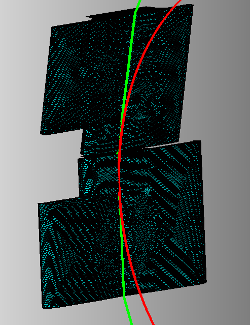
The following picture shows the shadowed, shadowing, LCFS and plasma geometry all together. The LCFS and plasma geometry were rotated by 70 degrees around the z axis.
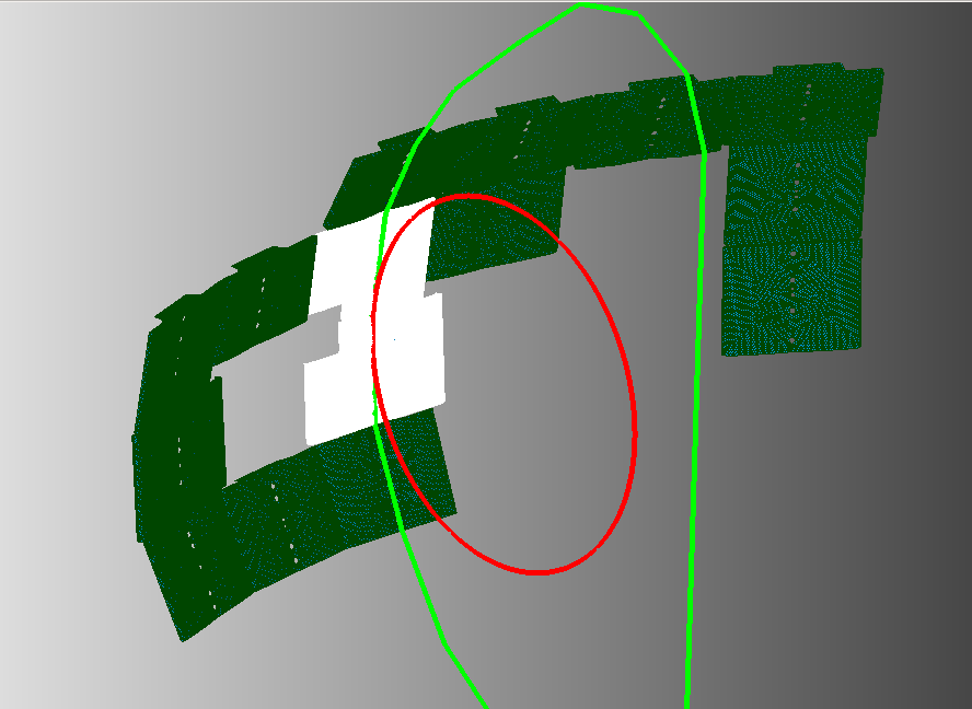
And a closed up image to the target NE14NE15 mesh.
4.15.3. Setting up the SMITER case
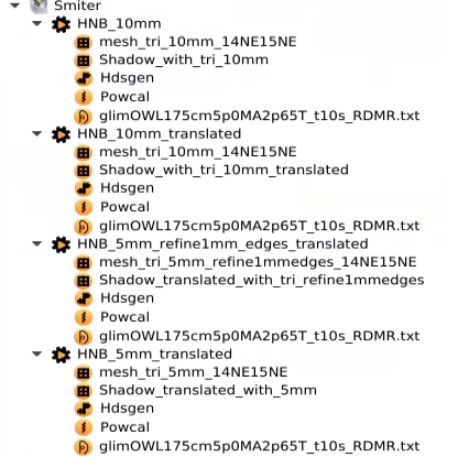
The study HNB.hdf already contains the meshes of the target panels and
shadow panels. Together the meshes of shadow panels are joined into a single
mesh called Shadow. Similarly the grouped mesh for translated shadows are
called Shadow_translated.
Since self-shadowing is also important, the final version of the shadow meshes are:
- Shadow_with_tri_10mm
- Shadow_with_tri_10mm_translated
4.15.3.1. Creating the SMITER case
When in SMITER, activate the SMITER module. Then click on the  to
open up the dialog.
to
open up the dialog.
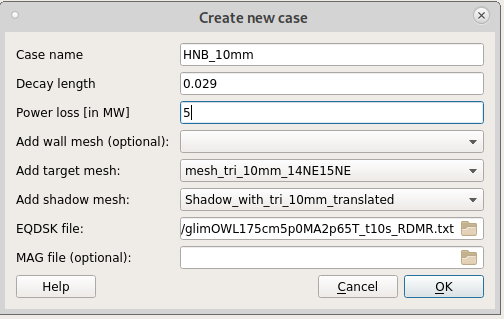
Set the Case name to HNB_10mm_translated. For this configuration the
decay length is 0.029 meters or 29 millimeters. The power loss defined is
to 5 MW. Leave the optional wall mesh empty and set the target mesh to
mesh_tri_10mm_14NE15NE and shadow mesh to
Shadow_with_tri_10mm_translated. For the EQDSK file click on the file
browser, set the Files of type to All files (*), go to
smiter/study/hnb and select glimOWL175cm5p0MA2p65T_t10s_RDMR.txt.
Click Ok.
4.15.3.2. Settings parameters for GEOQ
In the Salome Object browser right click on the target GEOQ, which has the same name as the target mesh. Select Edit CTL.
Under beqparameters change the parameters to the following values:
| Parameter | Value | Description |
|---|---|---|
| beq_bdryopt | 9 | Plasma flux value at boundary is given as input |
| beq_cenopt | 4 | Read the center values of R and Z from eqdsk file |
| beq_fldspec | 3 | Use Cartesian coordinate system |
| beq_nzetap | 1 | Fieldlines might go around torus! |
| beq_psiref | -13.6917 | Specify flux value at LCFS |
Note
The current beq_psiref is user specified, but the one written in the
EQDSK G file is -13.653458. The LCFS flux value depends on the geometry
of the target mesh.
Do the same for the shadow mesh.
Note
SMARDDA can evaluate the LCFS flux value with setting the beq_bdryopt to
3. But since it depends of type of interpolation (smardda uses a bivariate
spline) users might specify their own calculated value.
4.15.3.3. Setting parameters for HDSGEN
Right click on Hdsgen and select Edit CTL. Set the following
value under positionparameters.
| Parameter | Value | Description |
|---|---|---|
| position_transform | 1 | Scale in Cartesian coordinates |
Under btreeparameter set the following values.
| Parameter | Value | Description |
|---|---|---|
| tree_nxny | 1,2,2 | Multi-octree no. of children |
| tree_ttalg | 2 | Use nxyz, set split at top directly |
| tree_type | 3 | Type of tree is multi-octree |
Under hdsgenparameters set the following values.
| Parameter | Value | Description |
|---|---|---|
| geometrical_type | 2 | Element type is triangles |
| limit_geobj_in_bin | 200 | Max number of geometrical objects per bin |
| margin_type | 2 | Expand global bounding box bin |
4.15.3.4. Setting parameters for POWCAL
Right click on Powcal and select Edit CTL. Set the following
values under powcalparameters.
| Parameter | Value | Description |
|---|---|---|
| calculation_type | global | ‘global’ shadowing by fieldlines which may wrap around torus |
| shadow_control | 1 | Enable shadowing |
Prepared the rest of the cases in almost exact manner, except the meshes are different. The other cases can be prepared by duplicating the first one, changing the case name and replacing the meshes:
- Case with 10 mm target mesh and misalignment is not applied to shadow mesh
- Case with 5 mm target mesh and misaligned shadow mesh
- Case with 5 mm + refined edges target mesh and misaligned mesh
4.15.3.5. Run case
Now right click on the HNB_10mm and select Compute case.
Next step is running with shifted EQDSK data in Z-axis. The reason behind
is to see how the wetted area and heat load deposition changes in regards of
the shift. The following values are applied in such steps:
| Plasma position | beq_zmove (mm) | beq_psiref (LCFS) |
|---|---|---|
| 500 | 500 | -13.871 |
| 400 | 400 | -13.823 |
| 300 | 300 | -13.775 |
| 200 | 200 | -13.726 |
| 100 | 100 | -13.679 |
| 0 | 0 | -13.6917 |
| -100 | -100 | -13.725 |
| -200 | -200 | -13.76 |
| -300 | -300 | -13.794 |
| -400 | -400 | -13.828 |
| -500 | -500 | -13.862 |
We could duplicate each case for such shift, but that will result in larger .hdf file, too much data used on the filesystem when running the cases.
Instead we can use the provided dialog under .
When activated we select a SMITER case from the SALOME object browser, select
which parameter we would like to change, in this case beq_zmove and provide
a space separated list of values for the parameter (beq_zmove) we wish to
change and a space separated list of of values for the Psiref. Both lists
must contain the same number of values to run.:
# beq_zmove values
500 400 300 200 100 0 -100 -200 -300 -400 -500
# beq_psiref values
-13.871 -13.823 -13.775 -13.726 -13.679 -13.6917 -13.725 -13.76 -13.794 -13.828 -13.862
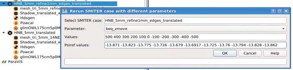
Then click Ok and the selected SMITER case will be rerun fully for all those values. This way we minimize the number of SMITER cases and therefore we minimize the risk of making small mistakes.
The output powcal_powx.vtk VTK file generated by POWCAL is saved as
<case_name>_<name_of_parameter>_<value_of_the_parameter>.vtk.
Therefore when the dialog finishes all the runs, activate ParaVis module,
and open the results as a ParaView group. This way instead of having
multiple pipeline objects in the VTK pipeline browser, you will have a grouped
object that has slide like functionality.
4.15.4. Results
4.15.4.1. Effect of misalignment on wetted area
The following images shows the importance of regarding misalignments on the shadow meshes. The images are for the case where no shift is applied to the EQDSK. It depends on what we focus, but for the base example, where no shift is added to the EQDSK, the wetted area changes on the center faces of the target.

Fig. 4.42 Importance of taking panel misalignment into account when it comes to shadowing effect
4.15.4.2. POWCAL results on HNB 5mm + refined edges meshes + misaligned shadow
The following images show the results of case with misaligned (or translated) shadow mesh and the 5mm + refined edges target mesh. The value shown of the images is the heat load Q \([\frac{MW}{m^2}]\).
The corresponding SMITER case in the HNB.hdf study is
HNB_5mm_refine1mm_edges_translated. For each case only the beqparameter
beq_zmove and beq_psiref is different. The results were obtained by
using the dialog to rerun cases at a different beq parameter and beq_psiref.

Fig. 4.43 Heat load profile for EQDSK shift > 0 along the z-axis
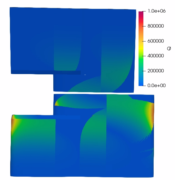
Fig. 4.44 EQDSK not shifted (beq_zmove=0, beq_psiref=-13.6917).

Fig. 4.45 Heat load profile for EQDSK shift > 0 along the z-axis
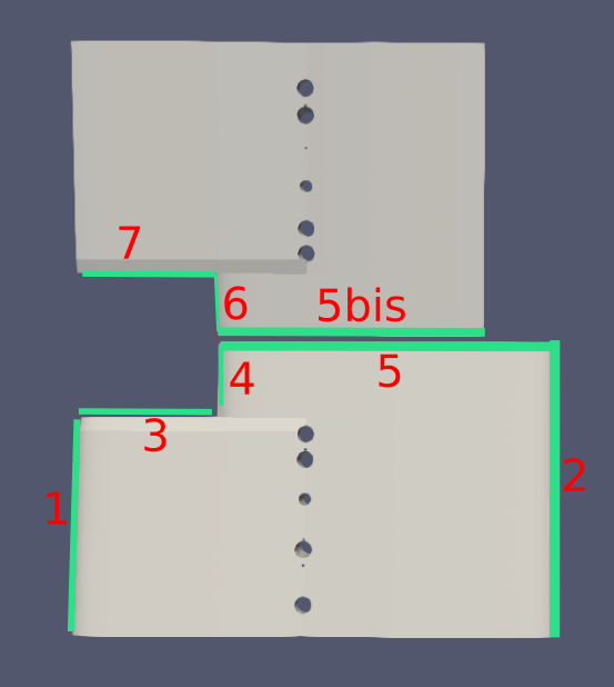
4.15.5. Edge results comparison
As in the reference study, the values will be shown for each edge and compared to the values in the study in the SMITER/PFCFLUX value.
The tables show heat deposition values and penetration length in dependence of EQDSK shift along the z-axis.
The values were taken inside ParaVis module. For \(q_{edge-Be}\) the
maximum value was taken right at the edge on the outer side. While for
\(q_{edge-Steel}\) the maximum value was taken at penetration length
20 millimeters. The way the penetration length was taken was to measure the
maximum achieved depth at each edge. If the specified value is Full or
Full edge then the wetted are is along the whole edge.
4.15.5.2. Edge #1
| beq_psiref (mm) | \(q_{edge-Be} [\frac{MW}{m^2}]\) | \(q_{edge-Steel} [\frac{MW}{m^2}]\) | penetration length (mm) |
|---|---|---|---|
| 500 | / | / | / |
| 400 | / | / | / |
| 300 | / | / | / |
| 200 | / | / | / |
| 100 | 0.39 / 0.33 | 0.24 / 0.2 | Full edge / Full edge |
| 0 | 0.58 / 0.5 | 0.25 / 0.29 | Full edge / Full edge |
| -100 | 0.58 / 0.5 | 0.24 / 0.23 | Full edge / Full edge |
| -200 | 0.58 / 0.5 | 0.24 / 0.23 | 30 mm / 30 mm |
| -300 | / | / | / |
| -400 | / | / | / |
| -500 | / | / | / |
4.15.5.3. Edge #2
| beq_psiref (mm) | \(q_{edge-Be} [\frac{MW}{m^2}]\) | \(q_{edge-Steel} [\frac{MW}{m^2}]\) | penetration length (mm) |
|---|---|---|---|
| 500 | / | / | / |
| 400 | / | / | / |
| 300 | / | / | / |
| 200 | / | / | / |
| 100 | / | / | / |
| 0 | 0.6 / 0.6 | 0.3 / 0.33 | 35 / 30 |
| -100 | 0.6 / 0.6 | 0.3 / 0.33 | Full / Full |
| -200 | 0.6 / 0.6 | 0.3 / 0.33 | Full / Full |
| -300 | 0.6 / 0.6 | 0.3 / 0.33 | Full / Full |
| -400 | 0.61 / 0.6 | 0.29 / 0.33 | Full / Full |
| -500 | 0.61 / 0.6 | 0.31 / 0.33 | Full / Full |
4.15.5.4. Edge #3
| beq_psiref (mm) | \(q_{edge-Be} [\frac{MW}{m^2}]\) | \(q_{edge-Steel} [\frac{MW}{m^2}]\) | penetration length (mm) |
|---|---|---|---|
| 500 | / | / | / |
| 400 | / | / | / |
| 300 | / | / | / |
| 200 | / | / | / |
| 100 | / | / | / |
| 0 | / | / | / |
| -100 | 1.38 / 1.3 | / | ~2 / 2 |
| -200 | 0.9 / 1.0 | / | 10 / 10 |
| -300 | 0.55 / 0.55 | / | 13 / 10-15 |
| -400 | 0.29 / 0.35 | 0.2 / 0.19 | 20 / 20 |
| -500 | 0.125 / 0.15 | 0.08 / 0.07 | 25 / 25 |
4.15.5.5. Edge #4
| beq_psiref (mm) | \(q_{edge-Be} [\frac{MW}{m^2}]\) | \(q_{edge-Steel} [\frac{MW}{m^2}]\) | penetration length (mm) |
|---|---|---|---|
| 500 | / | / | / |
| 400 | / | / | / |
| 300 | 0.15 / 0.15 | 0.09 / 0.09 | Full / Full |
| 200 | 0.3 / 0.3 | 0.2 / 0.2 | 35 / 35 |
| 100 | 0.6 / 0.6 | / | 15 / 15 |
| 0 | / | / | / |
| -100 | / | / | / |
| -200 | / | / | / |
| -300 | / | / | / |
| -400 | / | / | / |
| -500 | / | / | / |
4.15.5.6. Edge #5
| beq_psiref (mm) | \(q_{edge-Be} [\frac{MW}{m^2}]\) | \(q_{edge-Steel} [\frac{MW}{m^2}]\) | penetration length (mm) |
|---|---|---|---|
| 500 | / | / | / |
| 400 | / | / | / |
| 300 | / | / | / |
| 200 | / | / | / |
| 100 | / | / | / |
| 0 | 0.87 / 0.95 | / | 5 / 5 |
| -100 | 0.5 / 0.55 | / 0.27 | 18 / 20 |
| -200 | 0.2 / 0.27 | 0.1 / 0.13 | 27 / 25 |
| -300 | 0.09 / 0.1 | < 0.04 / 0.05 | 37 / 30 |
| -400 | / | / | / |
| -500 | / | / | / |
4.15.5.7. Edge #5 bis
| beq_psiref (mm) | \(q_{edge-Be} [\frac{MW}{m^2}]\) | \(q_{edge-Steel} [\frac{MW}{m^2}]\) | penetration length (mm) |
|---|---|---|---|
| 500 | / | / | / |
| 400 | 0.15 / 0.16 | 0.055 / 0.05 | > 50 / >>40 |
| 300 | 0.36 / 0.4 | 0.11 / 0.11 | > 50 / >>40 |
| 200 | 0.71 / 0.8 | 0.23 / 0.23 | 50 / > 40 |
| 100 | 1.14 / 1.35 | 0.35 / 0.35 | 25 / 25 |
| 0 | 0.9 / 0.9 | / | 10 / 10 |
| -100 | / | / | / |
| -200 | / | / | / |
| -300 | / | / | / |
| -400 | / | / | / |
| -500 | / | / | / |
4.15.5.8. Edge #6
| beq_psiref (mm) | \(q_{edge-Be} [\frac{MW}{m^2}]\) | \(q_{edge-Steel} [\frac{MW}{m^2}]\) | penetration length (mm) |
|---|---|---|---|
| 500 | 0.3 / 0.4 | 0.18 / 0.17 | Full / Full |
| 400 | 0.55 / 0.5 | 0.35 / 0.35 | Full / Full |
| 300 | 0.9 / 1 | 0.5 / 0.5 | 35 / 40 |
| 200 | 1.04 / 1.15 | / | 11 / 10 |
| 100 | / | / | / |
| 0 | / | / | / |
| -100 | / | / | / |
| -200 | / | / | / |
| -300 | / | / | / |
| -400 | / | / | / |
| -500 | / | / | / |
4.15.5.9. Edge #7
| beq_psiref (mm) | \(q_{edge-Be} [\frac{MW}{m^2}]\) | \(q_{edge-Steel} [\frac{MW}{m^2}]\) | penetration length (mm) |
|---|---|---|---|
| 500 | 0.3 / 0.3 | 0.15 / 0.2 | Full / Full |
| 400 | 0.55 / 0.6 | 0.35 / 0.4 | Full / Full |
| 300 | 0.85 / 0.8 | 0.45 / 0.4 | 65 / 65 |
| 200 | 1 / 1 | 0.6 / 0.65 | 35 / 30 |
| 100 | 1.1 / 1.1 | / | 9 / 7 |
| 0 | / | / | / |
| -100 | / | / | / |
| -200 | / | / | / |
| -300 | / | / | / |
| -400 | / | / | / |
| -500 | / | / | / |