4.11. Plugins¶

Plugins are available at Tools‣Plugins.

4.11.1. Writing plugins¶

Plugins in SALOME are python function that are run from the Tools ‣ Plugins menu.

The only difference between Load script from the File menu and the python plugins is the accessibility. While you need to remember where your script is saved, if you write a plugin function and store it inside the plugin python script, it will always be loaded and waiting for you in the Tools ‣ Plugins menu.

To write a python script and save it as plugin, you need to find the Plugins/ folder inside the source code of SMITER module, i.e.: SMITER/src/Plugins

There you will find a file named salome_plugins.py. To write your own functions you have to edit the file and add the following:

def your_fun(context):
    """The context contains the handle to other objects such as study,
    desktop object, etc... I.e.:
    study = context.study
    desktop = context.sg
    """
    your code

# In the end you need to register the function with:
salome_pluginsmanager.AddFunction('A name', 'Short description', your_fun)

Of course while the context handle provides the connections, you can easily import salome or other salome modules to find and process the data saved in the objects manager. Or you can create new objects, assign new attributes…

Note

Be careful if you have other functions defined outside of your function. Those functions need to be globalised before being called.

4.11.2. Create Divertor Mesh¶

This plugin creates divertor mesh that was used in Heat loads to the ITER first-wall panels for the ICRH-optimized plasma equlibrium written by dr. Martin Kocan. This divertor can be used for further studies in SMITER environment.

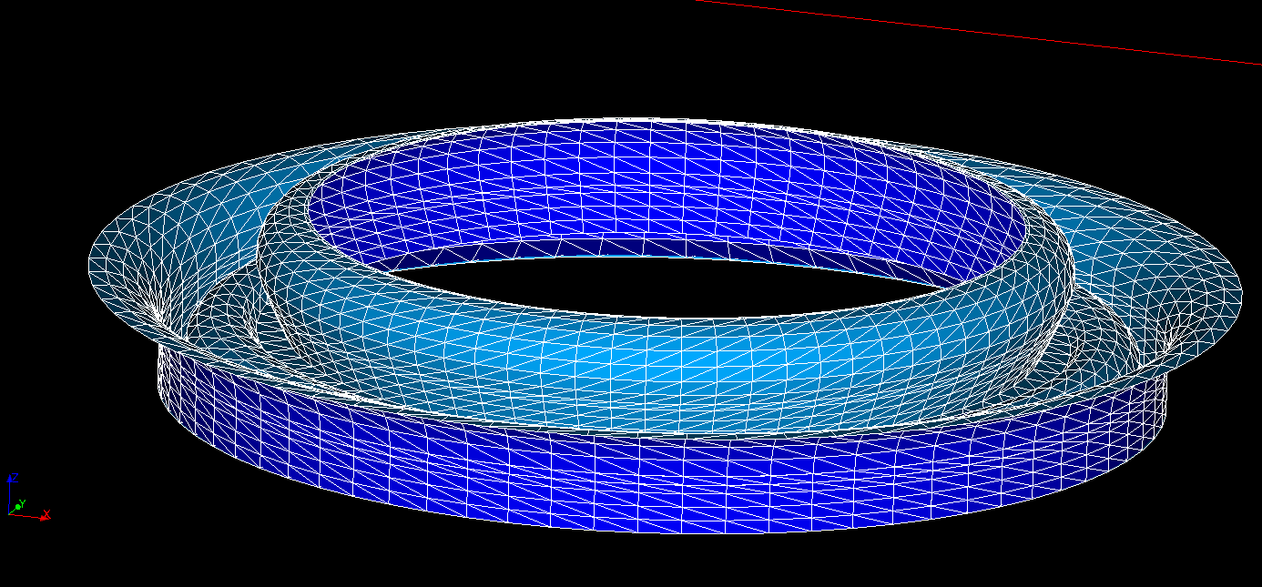
Fig. 4.30 Divertor.

4.11.3. Save fieldlines to HDF5¶

To activate fieldline plotting, navigate to powcal code in SMITER module and then open plot_selections and select flinx (Fieldlines in Cartesian coordinates) or flinm (Fieldlines in Flux-mapped coordinates). Fieldline for each mesh element in Cartesian or Flux-mapped coordinates is stored in form of .vtk file. If there are $N$ mesh elements, that means $N$ .vtk files. To reduce number of files, Save fieldlines to HDF5 Plugin can be used. This is a suitable options for storing and data transfer. When you click on Save fieldlines to HDF5, following dialog appears on screen.

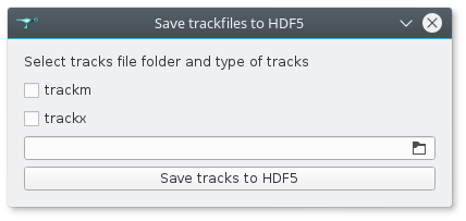
Fig. 4.31 Dialog for storing fieldlines to HDF5.

First you can select which type of fieldlines (trackm, trackx or both) you want to store to HDF5. Then select directory that contains fieldline .vtk files. With click on button Save tracks to HDF5 fieldlines will be stored to the same folder with two files. First file is tracksxHDF5.h5 (or tracksmHDF5.h5). This file contains coordinates of all fieldlines. Second file is tracksxHDF5.xdmf (or tracksxHDF5.xdmf). This file contains information on how Paraview should read HDF5 file and it contains information about polylines that form fieldlines.

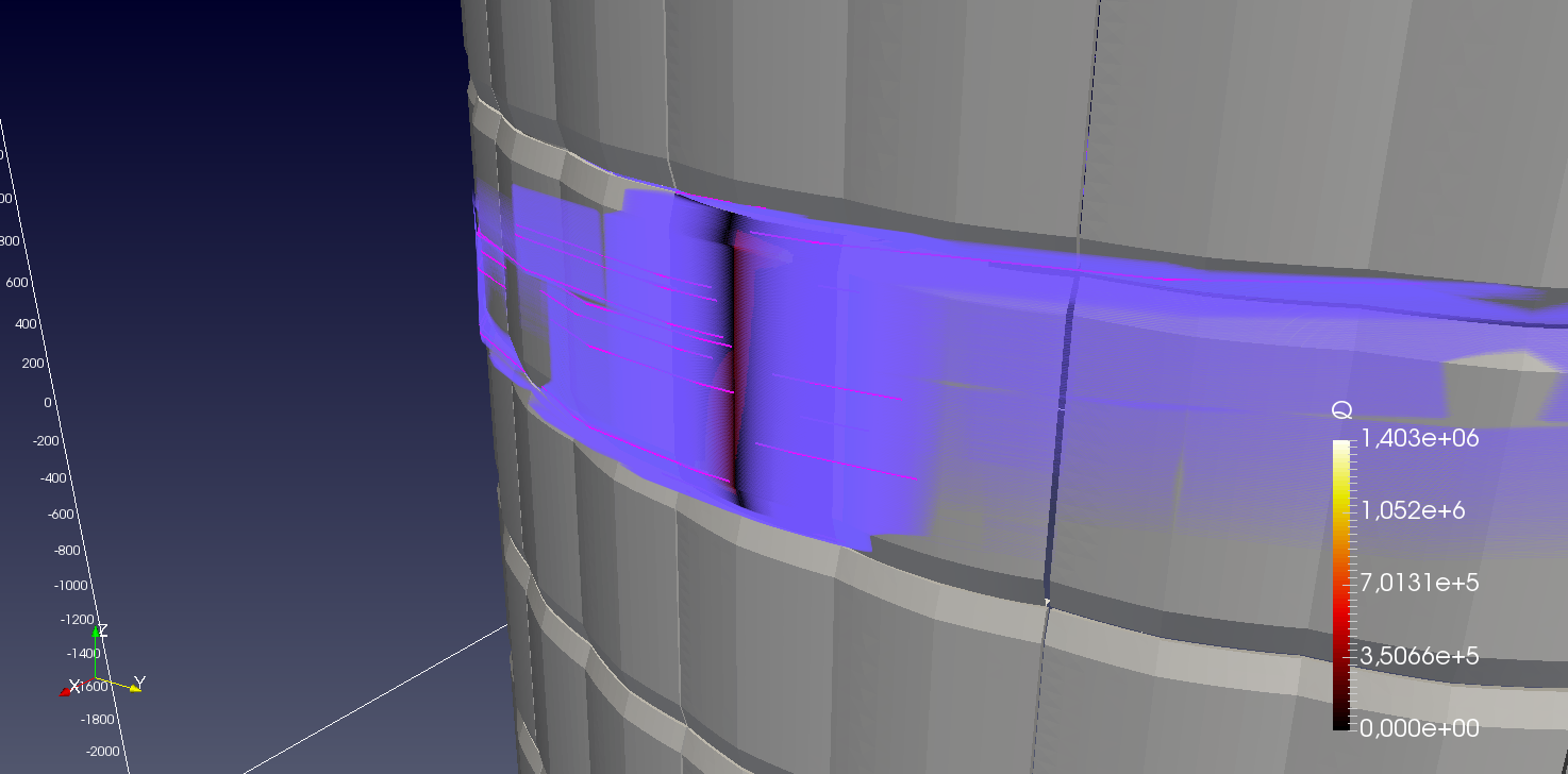
Fig. 4.32 Fieldlines in Cartesian coordinates.

4.11.4. Convert Energopul data format to MAG¶

This plugin converts Energopul data format into MAG format that can be used in cases with the presence of ripple field.

4.11.4.1. Energopul Format¶

Energopul files contain 3D database of magnetic field produced inside the vacuum vessel by the nominal current flowing in the toroidal field (TF) coils. The whole 3D database is divided in eighteen $20^\circ$ toroidal segments. It should be noted, that the notion “segment” is interpreted as a $20^\circ$ toroidal sector, $\pm 10^\circ$ from the poloidal midplane of corresponding TF coil.

The number of nodes assumes that in the poloidal plane the mesh boundary has rectangular cross section. This boundary is defined as follows: $r_{min}=3.7m$, $r_{max}=8.7m$, $z_{min}=-5.0m$, $z_{max}=+5.0m$. The error of field interpolation is estimated by subtracting the value of linear interpolation $(B_{r,i}-B_{r,i+1})/2$ and the real value at the center of the corresponding interval.

Therefore the following mesh were used for calculation of the database:

$3.7m \leqslant r \leqslant 8.7m$, step $\Delta r=0.1m$, 51 points in the radial direction

$-5.0m \leqslant z \leqslant 5.0m$, step $\Delta z=0.1m$, 101 points in the vertical direction

$\phi$ at $20$ º segment; step $\Delta \phi=(20/29)$, 30 points in the toroidal direction.

The obtained results for each segment have been presented in a file of 154530 strings with agreed format in the order of change: $R$, $Z$ and $\phi$ as it is shown in the table below:

String number	Content
1	$r_{1}\ \phi_{1}\ z_{1}\ B_r\ B_{\phi}\ B_z$
2	$r_{2}\ \phi_{1}\ z_{1}\ B_r\ B_{\phi}\ B_z$
…	…
51	$r_{51}\ \phi_{1}\ z_{1}\ B_r\ B_{\phi}\ B_z$
52	$r_{1}\ \phi_{1}\ z_{2}\ B_r\ B_{\phi}\ B_z$
…	…
102=5112	$r_{51}\ \phi_{1}\ z_{2}\ B_r\ B_{\phi}\ B_z$
103	$r_{1}\ \phi_{1}\ z_{3}\ B_r\ B_{\phi}\ B_z$
…	…
5151=511101	$r_{51}\ \phi_{1}\ z_{101}\ B_r\ B_{\phi}\ B_z$
5152	$r_{1}\ \phi_{2}\ z_{1}\ B_r\ B_{\phi}\ B_z$
5153	$r_{2}\ \phi_{2}\ z_{1}\ B_r\ B_{\phi}\ B_z$
…	…
154530=5130101	$r_{51}\ \phi_{30}\ z_{101}\ B_r\ B_{\phi}\ B_z$

As seen, each string contains six values separated by spacebars: three coordinates ($R$, $Z$ and $\phi$), and three field components ($B_r B_{\phi} B_z$), where $R$ and $Z$ are given in meters, $\phi$ - in degrees, magnetic field ($B_r B_{\phi} B_z$) - in Tesla.

The database is calculated assuming the value of current in each coil $I0=-9.128MA$ - turns, which produces at the radius $6.2m$ the nominal value of magnetic field $-5.3T$. This magnetic field has clockwise direction, when viewed from above.

4.11.4.2. Tutorial¶

To convert Energopul files to MAG format, activate SMITER module and navigate to Tools ‣ Plugins ‣ Energopul to MAG, as shown in Fig. 4.33. The dialog is shown in Fig. 4.34.

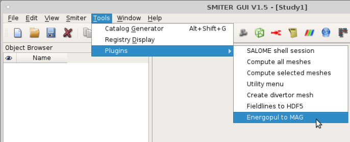
../_images/energopul_to_mag_navigation.png

Fig. 4.33 Navigation to plugin dialog.

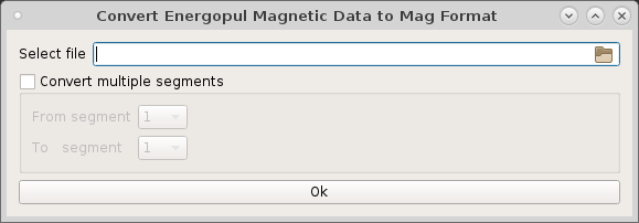
Fig. 4.34 Dialog to convert Energopul files to MAG format.

Click on the icon to open the file browser and navigate to the folder with Energopul files ($SMITER_STUDY_EXAMPLES_DIR/magtfm/TBM_6HZZEW_v1.2) and select the one that needs to be converted to MAG format. After the user clicks OK, new MAG file is generated in the same folder.

If the user wants to convert multiple Energopul segments into one MAG file, tick Convert multiple segments. See Fig. 4.35.

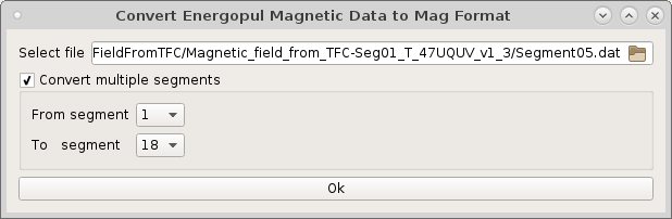
../_images/energopul_to_mag_multiple_seg.png

Fig. 4.35 Dialog to convert multiple Energopul files to MAG format.

Option Convert multiple segments reads multiple segments (In this case from Segment01.dat to Segment18.dat - refer to image Fig. 4.35) and creates one MAG file with all segments in the same folder.

Resulting file is takes basename without segment number with .txt extension. In our example this is Segment.txt.