4.22. Guide to Raysect samples

Author:David Križaj

The purpose of this report is to give users and developers of SMITER some basic information about Raysect module. The main reason is to inform users how changes in rendering parameters affect rendering quality and time which is needed to create an image. For this purpose we will use Cornell box example code from Raysect. For module presentation we will use the example code. The code will have some modifications for testing purposes.

4.22.1. Raysect basics

Raysect is an open-source python framework for geometrical optical simulations. Module is capable of creating realistic images with physical accuracy and high precision.

First we need to import functions from Raysect module. As seen in the code below we have to import all the functions we will use. Functions that need to be imported are in different classes. When we are importing the functions, we might consider importing them in a way that sorts them by the usage, even though functions may be from the same class.

from matplotlib.pyplot import *

from raysect.primitive import Sphere, Box
from raysect.optical import World, Node, translate, rotate, Point3D
from raysect.optical.material import Lambert, UniformSurfaceEmitter
from raysect.optical.library import *
from raysect.optical.observer import PinholeCamera
from raysect.optical.observer import RGBPipeline2D, BayerPipeline2D, PowerPipeline2D
from raysect.optical.observer import RGBAdaptiveSampler2D

After importing the needed functions, we can specify our material properties. For this we can use real measured data. All we need to know is the reflection percentage at different wavelengths of light. Measured data can be written in two 1D arrays, as we can see in the code below. Data, which is shown below, is actual data from measurements of a real Cornell box.

# define reflectivity for box surfaces
wavelengths = array(
  [400, 404, 408, 412, 416, 420, 424, 428, 432, 436, 440, 444, 448, 452, 456, 460, 464, 468, 472, 476, 480, 484, 488,
   492, 496, 500, 504, 508, 512, 516, 520, 524, 528, 532, 536, 540, 544, 548, 552, 556, 560, 564, 568, 572, 576, 580,
   584, 588, 592, 596, 600, 604, 608, 612, 616, 620, 624, 628, 632, 636, 640, 644, 648, 652, 656, 660, 664, 668, 672,
   676, 680, 684, 688, 692, 696, 700])

white = array(
  [0.343, 0.445, 0.551, 0.624, 0.665, 0.687, 0.708, 0.723, 0.715, 0.71, 0.745, 0.758, 0.739, 0.767, 0.777, 0.765,
   0.751, 0.745, 0.748, 0.729, 0.745, 0.757, 0.753, 0.75, 0.746, 0.747, 0.735, 0.732, 0.739, 0.734, 0.725, 0.721,
   0.733, 0.725, 0.732, 0.743, 0.744, 0.748, 0.728, 0.716, 0.733, 0.726, 0.713, 0.74, 0.754, 0.764, 0.752, 0.736,
   0.734, 0.741, 0.74, 0.732, 0.745, 0.755, 0.751, 0.744, 0.731, 0.733, 0.744, 0.731, 0.712, 0.708, 0.729, 0.73,
   0.727, 0.707, 0.703, 0.729, 0.75, 0.76, 0.751, 0.739, 0.724, 0.73, 0.74, 0.737])

green = array(
  [0.092, 0.096, 0.098, 0.097, 0.098, 0.095, 0.095, 0.097, 0.095, 0.094, 0.097, 0.098, 0.096, 0.101, 0.103, 0.104,
   0.107, 0.109, 0.112, 0.115, 0.125, 0.14, 0.16, 0.187, 0.229, 0.285, 0.343, 0.39, 0.435, 0.464, 0.472, 0.476, 0.481,
   0.462, 0.447, 0.441, 0.426, 0.406, 0.373, 0.347, 0.337, 0.314, 0.285, 0.277, 0.266, 0.25, 0.23, 0.207, 0.186,
   0.171, 0.16, 0.148, 0.141, 0.136, 0.13, 0.126, 0.123, 0.121, 0.122, 0.119, 0.114, 0.115, 0.117, 0.117, 0.118, 0.12,
   0.122, 0.128, 0.132, 0.139, 0.144, 0.146, 0.15, 0.152, 0.157, 0.159])

red = array(
  [0.04, 0.046, 0.048, 0.053, 0.049, 0.05, 0.053, 0.055, 0.057, 0.056, 0.059, 0.057, 0.061, 0.061, 0.06, 0.062, 0.062,
   0.062, 0.061, 0.062, 0.06, 0.059, 0.057, 0.058, 0.058, 0.058, 0.056, 0.055, 0.056, 0.059, 0.057, 0.055, 0.059,
   0.059, 0.058, 0.059, 0.061, 0.061, 0.063, 0.063, 0.067, 0.068, 0.072, 0.08, 0.09, 0.099, 0.124, 0.154, 0.192,
   0.255, 0.287, 0.349, 0.402, 0.443, 0.487, 0.513, 0.558, 0.584, 0.62, 0.606, 0.609, 0.651, 0.612, 0.61, 0.65, 0.638,
   0.627, 0.62, 0.63, 0.628, 0.642, 0.639, 0.657, 0.639, 0.635, 0.642])

We can see the reflectivity spectrum of enclosure walls on a figure below.

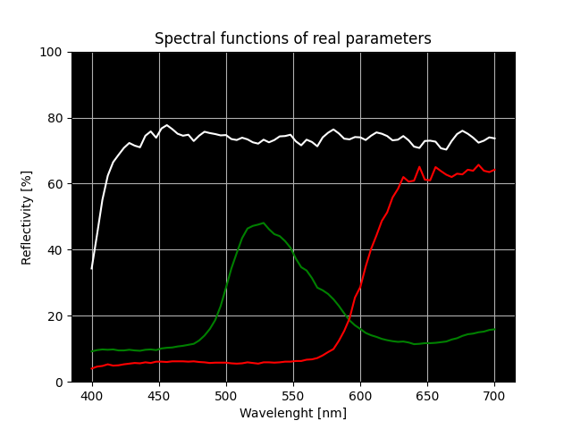
Fig. 4.103 White, red and green wall reflectivity spectrum.

To actually use this data we have to use the function InterpolatedSF().

white_reflectivity = InterpolatedSF(wavelengths, white)
red_reflectivity = InterpolatedSF(wavelengths, red)
green_reflectivity = InterpolatedSF(wavelengths, green)

After properties of our objects are defined, we need to set the scenography. Raysect scenography is created from nodes. Nodes are basic elements of scene-graph tree. Root node is created with the function World(). World node tracks all primitives and observers in the Raysect world. Other nodes can be used for combined objects like walls of the enclosure. Coordinate system used in Raysect is the Cartesian coordinate system.

# set-up scenegraph
world = World()

# enclosing box
enclosure = Node(world)

e_back = Box(Point3D(-1, -1, 0), Point3D(1, 1, 0),
            parent=enclosure,
            transform=translate(0, 0, 1) * rotate(0, 0, 0),
            material=Lambert(white_reflectivity))

e_bottom = Box(Point3D(-1, -1, 0), Point3D(1, 1, 0),
            parent=enclosure,
            transform=translate(0, -1, 0) * rotate(0, -90, 0),
            material=Lambert(white_reflectivity))

e_top = Box(Point3D(-1, -1, 0), Point3D(1, 1, 0),
            parent=enclosure,
            transform=translate(0, 1, 0) * rotate(0, 90, 0),
            material=Lambert(white_reflectivity))

e_left = Box(Point3D(-1, -1, 0), Point3D(1, 1, 0),
            parent=enclosure,
            transform=translate(1, 0, 0) * rotate(-90, 0, 0),
            material=Lambert(red_reflectivity))

e_right = Box(Point3D(-1, -1, 0), Point3D(1, 1, 0),
            parent=enclosure,
            transform=translate(-1, 0, 0) * rotate(90, 0, 0),
            material=Lambert(green_reflectivity))

# ceiling light
light = Box(Point3D(-0.4, -0.4, -0.01), Point3D(0.4, 0.4, 0.0),
          parent=enclosure,
          transform=translate(0, 1, 0) * rotate(0, 90, 0),
          material=UniformSurfaceEmitter(light_spectrum, 2))

# objects in enclosure
box = Box(Point3D(-0.4, 0, -0.4), Point3D(0.3, 1.4, 0.3),
          parent=world,
          transform=translate(0.4, -1 + 1e-6, 0.4)*rotate(30, 0, 0),
          material=schott("N-BK7"))

sphere = Sphere(0.4,
          parent=world,
          transform=translate(-0.4, -0.6 + 1e-6, -0.4)*rotate(0, 0, 0),
          material=schott("N-BK7"))

Cornell box scenography consists of two nodes. First node is a world, and second node is an enclosure. The enclosure is created with the function Node() and is part of the world node. The enclosure node consists of six objects. There are five walls and one light source. The enclosure node is shown on a figure below. We define the node which an object is connected to using the parameter parent. Position of the objects is defined with parameter transform. Transform is defined by two functions, translate() and rotate(). To understand how these two functions affect the position of the objects, we have to know in which way the axis of the coordinate system are pointing. The coordinate system is shown on a figure below.

Material type of the object is defined with the parameter material. Raysect already has a library of materials or colors that can be used with different surface effects.

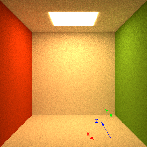
Fig. 4.104 The enclosure node with the Cartesian coordinate system orientation.

After the composition is all set, we have to define the rendering settings, as shown in a code block below.

filter_red = InterpolatedSF([100, 650, 660, 670, 680, 800], [0, 0, 1, 1, 0, 0])
filter_green = InterpolatedSF([100, 530, 540, 550, 560, 800], [0, 0, 1, 1, 0, 0])
filter_blue = InterpolatedSF([100, 480, 490, 500, 510, 800], [0, 0, 1, 1, 0, 0])

# create and setup the camera
power_unfiltered = PowerPipeline2D(display_unsaturated_fraction=0.96, name="Unfiltered")
power_unfiltered.display_update_time = 15

power_green = PowerPipeline2D(filter=filter_green, display_unsaturated_fraction=0.96, name="Green Filter")
power_green.display_update_time = 15

power_red = PowerPipeline2D(filter=filter_red, display_unsaturated_fraction=0.96, name="Red Filter")
power_red.display_update_time = 15

rgb = RGBPipeline2D(display_unsaturated_fraction=0.96, name="sRGB")

bayer = BayerPipeline2D(filter_red, filter_green, filter_blue, display_unsaturated_fraction=0.96, name="Bayer Filter")
bayer.display_update_time = 15

pipelines = [rgb, power_unfiltered, power_green, power_red, bayer]

sampler = RGBAdaptiveSampler2D(rgb, ratio=10, fraction=0.2, min_samples=500, cutoff=0.01)

First, we need to set the RGB filters. Filters are used to be multiplied with a measured power spectrum. By doing that, we get rid of some false samples, which are out of our filter range. Then we need to set how we would like to present our measurements. For that we need the pipeline functions. The pipeline functions are like camera settings when you are taking a photograph with a camera. For 2D images, we can use the PowerPipeline2D() function. With the parameter display_update_time we can set the rendering update time. This setting is useful when render needs a lot of time for every render pass. After every render pass there is always an update of the displayed image. After all our pipelines are set, we put them in a list of pipelines that will come in use later.

After all our pipelines are set, we have to define how we would like to sample our objects. For that purpose a sampler function is used. Raysect enables us to sample in two ways. For 2D sampling we can use FullFrameSampler2D() that evenly samples the whole image, or we can use other adaptive sampling methods. For images we use RGBAdaptiveSampler2D(). Sampler settings have the main impact on rendering time and rendering quality. The impact of sampler settings is presented in a paragraph below.

After sampling and presentation settings are all set, there is a need to place observer in a right place to make sure all things are caught in the observers view. There are a few types of observers which can be used. For creating realistic images the best type of the observer to use is PinholeCamera(). It gives us the perspective and we can set the viewing angle of the camera. Default angle is set to 45 degrees. How to set the observer is shown in a code block below.

camera = PinholeCamera((1024, 1024), parent=world,
transform=translate(0, 0, -3.3) * rotate(0, 0, 0), pipelines=pipelines)
camera.frame_sampler = sampler
camera.spectral_rays = 1
camera.spectral_bins = 15
camera.pixel_samples = 250
camera.ray_importance_sampling = True
camera.ray_important_path_weight = 0.25
camera.ray_max_depth = 500
camera.ray_extinction_min_depth = 3
camera.ray_extinction_prob = 0.01

The first thing that needs to be defined is the resolution of the created image. To set the image resolution we have to set the number of pixels in X and Y direction. Then we define the parent node of the observer and the position of the observer in the Raysect world. Default normal vector of the observer is pointing in Z direction. When the observer is placed, we need to define what type of spectrum we would like to observe. For that purpose we set the parameter pipelines to the list of pipelines we created before. After that, we set the type of sampler we would like to use. Then we can adjust some other parameters, for example the number of bins that the spectrum will be divided into for statistical purposes with the parameter spectral_bins. Or we can adjust the number of samples to take per pixel with pixel_samples.

All we need now is a part of the code to start creating an image and saving it.

# start ray tracing
ion()
name = 'cornell_box'
timestamp = time.strftime("%Y-%m-%d_%H-%M-%S")
render_pass = 1
while not camera.render_complete:

    print("Rendering pass {}...".format(render_pass))
    camera.observe()
    rgb.save("{}_{}_pass_{}.png".format(name, timestamp, render_pass))
    print()

    render_pass += 1

ioff()
rgb.display()

Rendering starts with ion() and ends with ioff(). Between that we need to put a loop that will run until parameters we set above are fulfilled.

4.22.2. Raysect benchmarking

Raysect (raysect.org) has numerous influential parameters that control image accuracy and overall time. We have to deal with two main parameters:

• ratio
• cutoff

We will be using default examples to explain these for PFC relevant models.

For analysis purposes we will use the example from raysect.org page. Default code can be found at:

cd examples/raysect
../../smiter -t cornell_box.py

4.22.2.1. Cutoff

Cutoff is a parameter which controls image noise. Parameter value should be between 0 and 1. When image noise is under the set threshold, program will abort extra sampling and complete the rendering process.

On figure below we can see how the cutoff setting affects image quality. All images have the ratio set to 2.

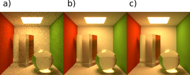
Fig. 4.105 Ratio = 2, cutoff settings are a) cutoff = 1, b) cutoff = 0.1, c) cutoff = 0.025.

4.22.2.2. Ratio

The ratio parameter determines the maximum proportion between the number of samples received by a pixel with the most samples and the number of samples received by the pixel with the least number of them. These 2 pixels need to be from the same observer (camera). In order to keep the proportion below the set value, the sampler generates extra assignments for the pixels with minimal number of samples.

On a figure below we can see how the ratio setting affects image quality. All images have the cutoff set to 0.2.

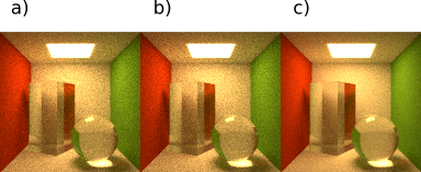
Fig. 4.106 Cutoff = 0.2, ratio settings are a) ratio = 200, b) ratio = 10, c) ratio = 2.

With lowering of the ratio parameter we also affect image quality in a way that reduces image noise.

4.22.2.3. Code

The test code was edited in a way that enables us to make tests with different parameters. The test code is located at:

cd examples/raysect
../../smiter -t raysect_testing.py

The program asks for the number of pixels in horizontal (X) and vertical (Y) direction. There is a need to insert the name of .txt file and then the file with the results is created.

Selected number of pixels affects the calculation time and the image quality. The following results were created with the image size of 128x128 pixels.

The results were created with these two lists of parameters:

list_s_ratio = [200, 150, 100, 50, 20, 10, 5, 2]
list_s_cutoff = [1, 0.95, 0.9, 0.85, 0.8, 0.75, 0.7, 0.65, 0.6, 0.55, 0.5,
                 0.45, 0.4, 0.35, 0.3, 0.25, 0.2, 0.15, 0.1, 0.05, 0.025]

With two for loops in the code all combinations can be tested and time measured. The created code is also capable of counting the number of passes.

Raysect package is created so that it accumulates rendering results. That means that by changing the cutoff parameter we just continue with rendering the current image, until we achieve set noise threshold.

By putting the pipeline function inside the ratio parameter setting for loop we start a new rendering process for every ratio setting. With this modification of the code we can provide the appropriate measurement for every specified setting combination. Shown test results were performed on Intel(R) Core(TM) i7-7500U with two cores. With a higher number of cores, we can estimate shorter rendering times.

On the figure below we can see how rendering time changes according to different rendering settings.

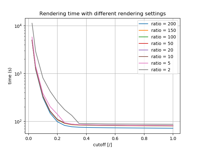
Fig. 4.107 Rendering time results with different ratio and cutoff settings. Y axis is in log scale.

4.22.2.4. Number of cores

The number of cores we are using should affect the rendering time in a way that using twice as much CPUs reduces rendering time by half. Raysect enables us to set the number of cores we would like to use. By default Raysect uses all available cores. If we want to specify the number of cores, we have to use Raysect function MulticoreEngine().

cores_num = [1, 2, 4, 8, 16, 32, 64, 128]
for i in cores_num:
  camera = PinholeCamera((x_res, y_res), parent=world,
  transform=translate(0, 0, -3.3) * rotate(0, 0, 0), pipelines=pipelines)
  camera.render_engine = MulticoreEngine(processes= i)
  camera.frame_sampler = sampler
  camera.spectral_rays = spectral_rays
  camera.spectral_bins = spectral_bins
  camera.pixel_samples = pixel_samples
  camera.ray_importance_sampling = ray_importance_sampling
  camera.ray_important_path_weight = ray_important_path_weight
  camera.ray_max_depth = ray_max_depth
  camera.ray_extinction_min_depth = ray_extinction_min_depth
  camera.ray_extinction_prob = ray_extinction_prob

With the parameter processes we set the number of cores we would like to use in our rendering process.

To test this we used HPC MAISTER from University of Maribor. A single MAISTER node has 128 core units. We decided to make tests with 1, 2, 4, …, 128 cores and a for loop, as seen on the code block above. For that purpose we created .sbatch file to use the whole node for our test.

#!/bin/bash
#SBATCH -n 128
#SBATCH -N 1
#SBATCH --time=32:00:00
#SBATCH --output=rsect128.out

mypython/bin/python raysect_testing_core_loop.py

Test file settings are:

• resolution: 128x128
• cutoff: 0.025
• ratio: 2

Rendering times are shown in a table below.

Table 4.3 Rendering times with different number of cores

Number of cores	1	2	4	8	16	32	64	128
Rendering time [s]	23852	11688	6078	3161	1872	1147	816	878

Results are also shown on the figure below.

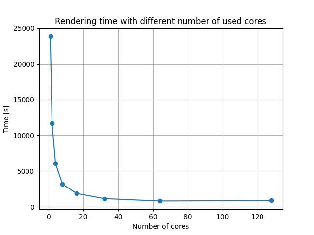
Fig. 4.108 Rendering time results with different number of cores used.

We had expected that rendering time would be halved, if we used twice as much core units. For easier presentation of time halving, figure below was created. Results show that our expectations were not entirely met.

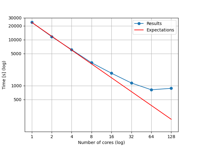
Fig. 4.109 Rendering times with different number of cores used and expected times of rendering in addition to rendering time with 1 core.

Our expectations were based on the time, which Raysect needed for rendering our example with only 1 CPU unit. Then we drew a line that our rendering times should follow, if we doubled the number of CPUs. As seen on the figure above, our actual results did not follow the expectations completely. The cause for this misalignment is that 128 cores are not actuall cores. 128 cores are virtually available because of hyper-threading option that HPC-RIVR CPUs can afford. If program is capable of hyper-threading, that option enables the time cut around 30%. Because Raysect is not capable of that, when we use all of the available cores and hyper-threading option, it actually takes more time to calculate in comparison to not using hyper-threading.

Our expectations were based on the time, which Raysect needed for rendering our example with only 1 CPU unit. Then we drew a line that our rendering times should follow, if we doubled the number of CPUs. As seen on the figure above, our actual results did not follow the expectations completely. The cause for this misalignment is that two CPU units share one memory unit. Because of that, one of the two units with the shared memory has to wait while the other one writes the information in shared memory. When we use all of the available cores, the effect of waiting is most significant. This leads to the fact, that rendering time with 128 cores is longer than one with 64 cores in use.