2.7. ITER NF55 Case

2.7.1. Introduction

In this tutorial, a benchmark study for SMITER environment will be presented. The starting point is an article Impact of a narrow limiter SOL heat flux channel on the ITER first wall panel shaping [NF55]. Power deposition and incidence angles on first wall panel 4 (FWP4) were studied in this NF55 paper with the field line tracing code PFCFLUX. The goal of the SMITER benchmark study is to repeat this PFCFLUX study in order to confirm the capability of SMITER as an appropriate solver for fieldline tracing and power deposition studies.

[NF55]

(1, 2, 3) Martin Kocan et al., Nucl. Fusion. 55 (2015) 033019 (16pp), doi:10.1088/0029-5515/55/3/033019

Note

This tutorial benchmark study does not resemble current ITER wall geometry and serves only as demonstration of SMITER capabilities for comparing to results found in Nuclear Fusion paper.

Fig. 2.2 Wall mesh and LCFS

In Fig. 2.2, the zoomed part on the left (a) represents the neighborhood of FWP4 from the first wall cross section (b). The first wall for FWP4 with radius R = 4.08m is shown as a light-green curve. Non-shifted equilibrium from DINA 15MA scenario, t=16.97s, Ip=5MA by Y. Gribov and last closed flux surface (LCFS) (light-blue curve) need to be shifted outwards for 25 mm to match the NF55 paper’s mesh (dark green area) and wall (light-green). The current (2017) wall mesh at R=4.105m, that is not used for this benchmark, is represented by a red curve.

2.7.2. Shadowing and Target description

The resulting study and meshes used in this study are available in SMITER directory smiter/salome/study/iter-nf55.

Study:

• nf_55_033019_2015.hdf, a complete study ready for a rerun. It is intended for comparison with the final results obtained at the end of this tutorial.

Meshes:

• FWP4_2lambdaOpt50mm4mmK4_asymmetric_with_edges.dat, a mesh used for target panels 3, 4 and 5,
• FWP4_2lambdaOpt50mm4mmK4_asymmetric_with_edges_rough_resolution.dat, a mesh used for shadow panels 3, 4 and 5,
• FWP1.dat, a mesh of shadow panel 1,
• FWP2.dat, a mesh of shadow panel 2,
• FWP6.dat, a mesh of shadow panel 6,
• FWP7.dat, a mesh of shadow panel 7.

All above listed meshes form and represent the new first wall shape and are the same meshes that were used in NF55 paper.

In order to redo the case from the report we need to first understand the shadow and target geometry used in PFCFLUX study. The shadow is shifted 5 mm away in radial direction from the center of the plasma to allow for thermal expansion of vessel under operating conditions. The shadow geometry and target used in the report are shown in Fig. 2.3. In this tutorial we will focus only on panel 4 as a target.

In SMITER it is required to have a shadow geometry that includes the target or final resulting geometry like in the test case Val-F11-fw264t-fw4t-1l. First wall panel 4 in ITER tokamak (including all other panels) consists of two subpanels that are shadowed by each other. To get the correct results the target too must shadow itself. Because of that, the target needs to be included in the shadow as well.

First, import the meshes into SMITER. Then radially move the shadow panels 5 mm away from plasma.

Note

To learn how to move the meshes in SMESH module, please refer to the section Using SMESH module‣Moving meshes in 3D space‣ Translating meshes.

With the shadow positioned correctly, the target is to be separated into the left and right subpanels.

Note

To learn how to split individual meshes into multiple meshes refer to section Using SMESH module‣Building submeshes.

Fig. 2.3 Panel FW4 (green) with shadowing geometry (white). Note that shadow is radially shifted away by 5 mm.

With the target ready, the next phase is to prepare the shadow. The shadow must contain all geometry that can intercept field-lines from the target/result geometry. Using the neighbouring panels as a shadow of panel 4 will result in an increased wetted area, the same as observed in the report. To achieve similar results it is necessary to include at least 5 neighbouring panels in the toroidal direction of ITER tokamak.

Note

To learn how to build compound out of multiple meshes, refer to Using SMESH module ‣ Building a Compound out of multiple Meshes.

As mentioned above, the target must be included in shadowing geometry to shadow itself. This can be achieved by first moving the shadowing target mesh away from plasma for a very short distance (approx. \(x_{tar shad}=-0.1mm\)) and then merge it with the shadow by using the Build Compound function. In case that this step is skipped a numerical error might occur during the computation, resulting in no power deposition on some triangles even though they are wetted, as shown in Fig. 2.4.

Note

There is a parameter to prevent this self-intersection under odesparameters called termination_parameters(1) that practically means the minimum connection lenght under which intersection test will not executed and next step is imediately continued. Recommended value for this parameter is the average length of triangles on the target mesh. In this case this is 5 mm or slightly larger termination_parameters(1) value.

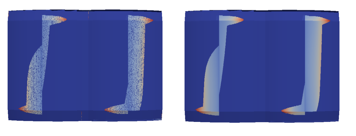
Fig. 2.4 Left: Possible numerical error if shadow overlaps target. Note that some triangles result in no power deposition despite being wetted. Right: Correct result with no numerical error.

2.7.2.1. Step by Step Instructions

The next steps will demonstrate how to prepare the full mesh needed for the study.

1. Import the meshes

To import all meshes available for the NF55 study use the NASTRAN to MESH option, as shown in Fig. 2.5.

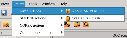
Fig. 2.5 Navigation to the NASTRAN to MESH option. From the top menu bar navigate to Smiter -> Mesh Actions -> NASTRAN to MESH.

Note

For more detailed description refer to Using SMITER GUI.

With the use of this function proceed to import the NASTRAN meshes FW4, FW1, FW2, FW6, and FW7. Then the meshes should be ready as shown in Fig. 2.6. For the purposes of this tutorial, it is advised to set the labels of those meshes to be the same as the names of the NASTRAN files.

Note

For more detailed instructions on how to import meshes into SMITER refer to Importing meshes video tutorial.

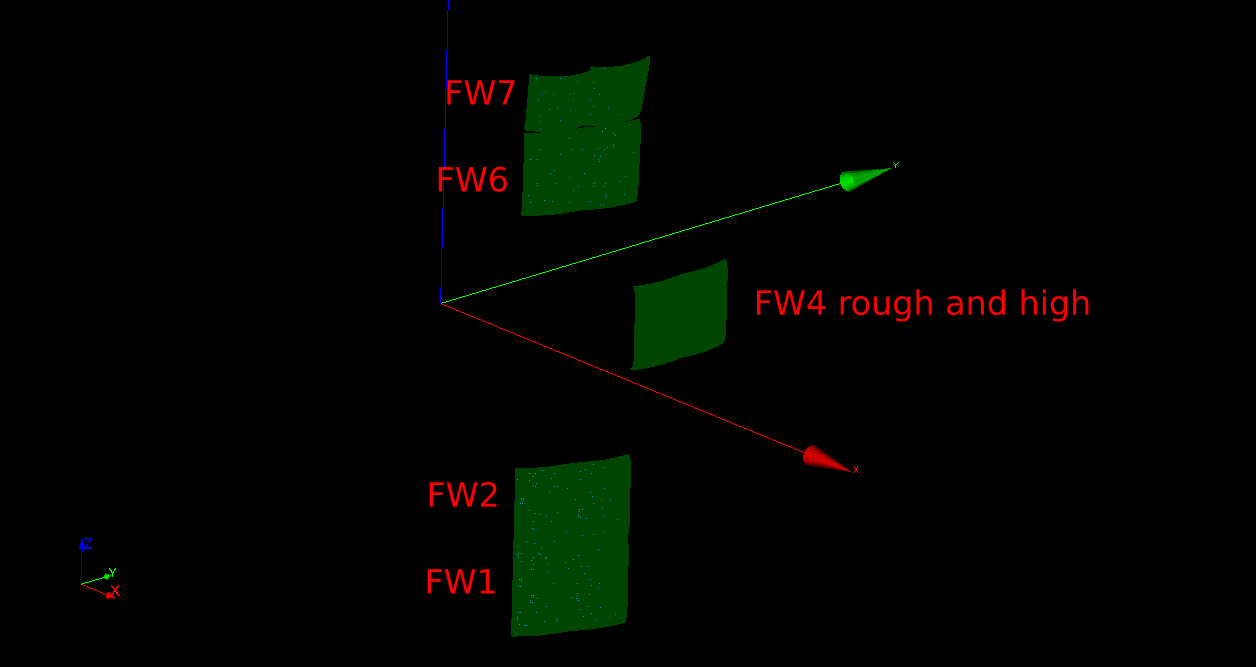
Fig. 2.6 All imported meshes, as seen in the SMITER-GUI Mesh module.

2. Copy the meshes

Proceed by copying the mesh (see Fig. 2.7) with a rough resolution for panel 4, used for shadowing, two times and move them in the Z-direction (see Fig. 2.8). Move the first mesh for \(\Delta z_5=+1015mm\) (this mesh will represent FWP5) and the second mesh for \(\Delta z_3=-1015mm\) (this mesh will represent FWP3). Rename those to meshes to _translatedplus1015 and _translatedminus1015.

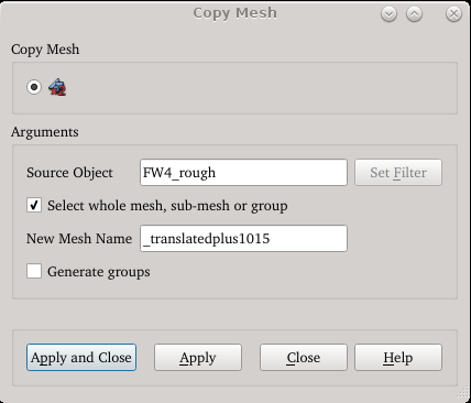
Fig. 2.7 Copy mesh procedure using the mesh of the panel 4 (rough): First select (left click) on the wanted mesh in the Mesh SMITER-GUI window, then run the Copy mesh tool . The tool window will be shown. Insert the required parameters and press the Apply button.

Then select panels 1, 2, 6 and 7 and combine them with the Build compound mesh tool to a mesh named FW1267 (see Fig. 2.9). After that rotate the FW1267 mesh for \(\Delta \phi=20\), so that the panels are positioned in \(x\) axis (see Fig. 2.10). Rename this new mesh to FW1267_rotatedplus20.

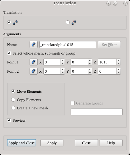
Fig. 2.8 Mesh translation procedure using the mesh of the copied panel 4: First select (left click) on the wanted mesh in the Mesh SMITER-GUI window. Then run the Translation tool . The tool window will be shown. Insert the required parameters and press the Apply button.

Fig. 2.9 Build compound mesh procedure using the mesh of the panels 1, 2, 6, and 7: Select (hold shift key + left ckick) the wanted meshes in the Mesh SMITER_GUI window. Then run the Build compound mesh tool . The tool window will be shown. Insert the required parameters and press the Apply button.

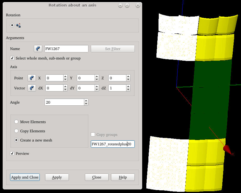
Fig. 2.10 Mesh rotation procedure using the mesh of the combined panels 1, 2, 6 and 7: First select (hold shift + left click) the wanted meshes in the Mesh SMITER-GUI window. Then run the Rotation tool . The tool window will be shown. Insert the required parameters and press the Apply button. The preview is shown as a yellow mesh.

Next, combine the FW1267_rotatedplus20, _translatedplus1015, _translatedminus1015 and FW4 (rough) meshes with the Build compound mesh* tool to a mesh named fullsegment (see Fig. 2.11).

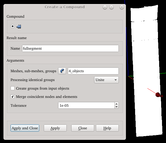
Fig. 2.11 Build compound mesh procedure: Select (hold shift key + left ckick) the wanted meshes in the Mesh SMITER_GUI window. Then run the Build compound mesh tool . The tool window will be shown. Insert the required parameters and press the Apply button.

Now one full segment, consisting of all panels from 1 to 7, should be ready, same as shown in Fig. 2.12.

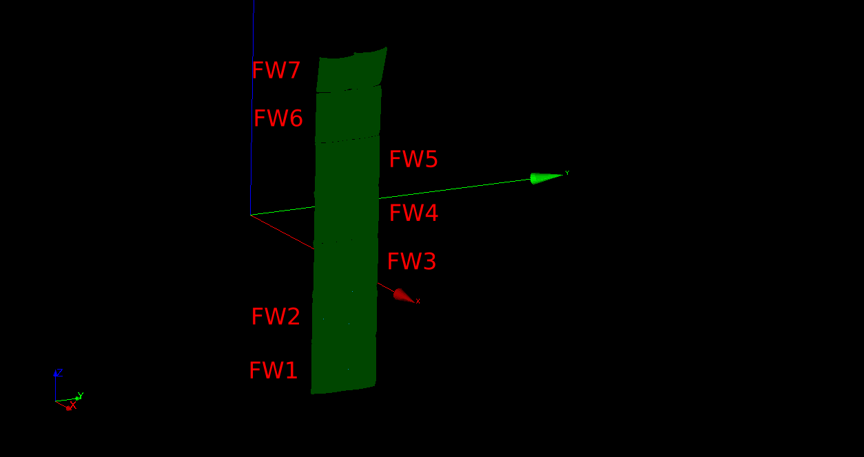
Fig. 2.12 One full segment.

3. Position and expand the shadow

Next, move the created full segment (study name fullsegment) 5 mm towards the coordinate system (\(\Delta r=-5mm\) or in cartesian coordinates \(\Delta x=-5mm\)) ( tool) and name this mesh fullsegment_translatedmin5. Then copy this segment in the toroidal direction for \(\Delta\varphi=20^\circ\) with respect to neighbouring segment (use and tools). The whole shadow should have 11 segments. One in the middle will contain a hole for the target and it should consist of only panels 1, 2, 3, 5, 6 and 7. The panel 4 is not included in this segment because FW4 is a target that is not moved back by \(-5mm\).

Next, use the Copy Mesh , Translate Mesh and Build a Compound tools to first combine the _translatedplus1015, _translatedminus1015 and FW1267_rotatedplus20 meshes into single mesh named fullsegmentNoFW4, then translate the same mesh for \(\Delta x=-5mm\). This segment is now surrounded by 5 neighbouring segments in both directions.

Then proceed to combine the fullsegmentNoFW4 and 10 neigbouring full segments meshes to shadowNoFW4 mesh. the final mesh is shown in Fig. 2.13

Note

Do not forget that the middle sector should not include first wall panel 4, so in the end, when merging panels into a single mesh, exclude panel 4 in the middle sector, same as shown in Fig. 2.13.

Note

For more detailed instructions on how to build and prepare full shadow refer to Transforming meshes for complete case video tutorial.

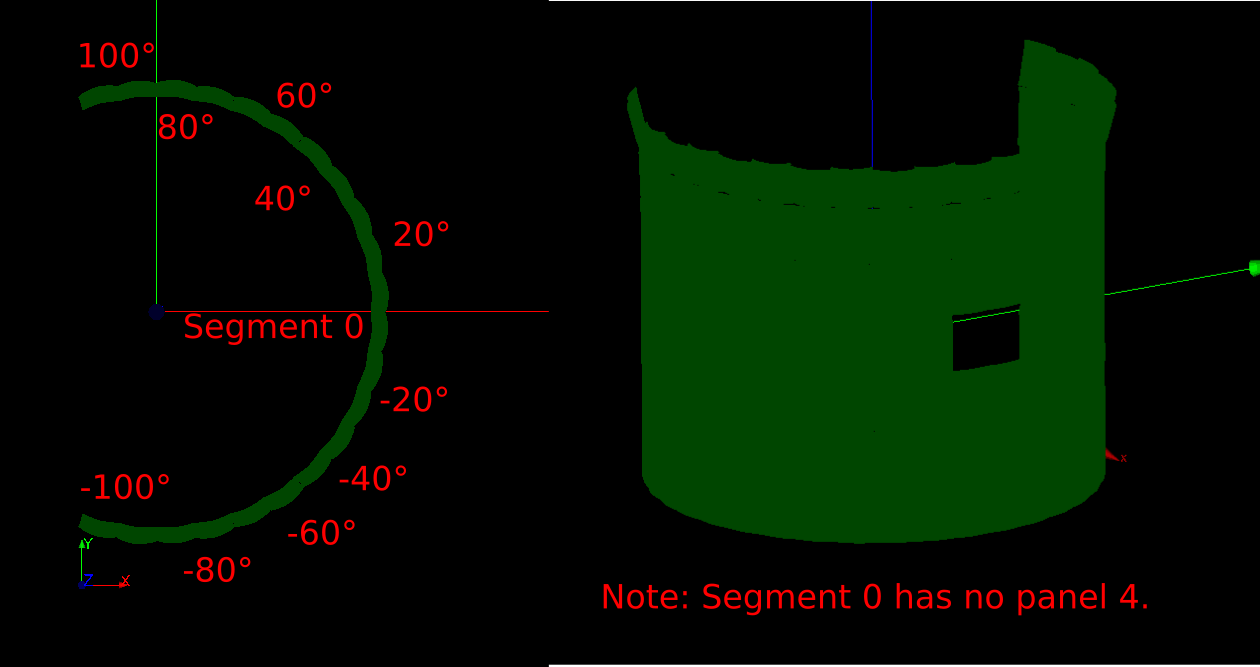
Fig. 2.13 Shadow for the NF55 case. The original segment is named Segment 0. All other neighbouring panels are created by copying and rotating this segment. Note that panel 4 is not included into shadow, because it is used as a target.

4. Include target panel into shadow

When shadow, as shown in Fig. 2.13, is obtained, the shadowing target (mesh with high resolution) can now be included. Import FW4 mesh with high resolution again and name it shadowingtarget. To avoid possible numerical errors, move the shadowing target for \(x_{tar shad}=-0.1mm\) and then merge the shadow and shadowing target with the Build Compound function. When that is done the full shadow is completed.

Note

The movement \(x_{tarshad}-0.1mm\) can be avoided by setting the POWCAL parameter, odesparameters::termination_parameters(1) to value 6. This sets the minimum length at which POWCAL does not check if a trajectory has hit anything. This parameter is set in Section 2.7.3.

5. Import target and wall mesh

Import FW4 mesh with high resolution again and this time name it target. Now both the full target and shadow are completed. The remaining task is to import the wall mesh named nf_55_033019 wall. Do that by, while in the Smiter module, navigating to Smiter -> Mesh actions -> Create wall mesh as shown in Fig. 2.14. A window with selection of wall meshed will be displayed. Select the nf_55_033019 option, as shown in Fig. 2.15.

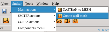
Fig. 2.14 Navigation to the SMITER-GUI Create wall mesh feature.

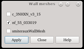
Fig. 2.15 Create wall mesh window and nf_55_033019 wall selection.

When that is done switch to Smiter module to create the NF55 case.

2.7.3. Study Parameters

According to the PFCFLUX paper, input parameters for the case are (see also Fig. 2.16):

• Power loss \(P\) = 5 MW
• Decay length \(\lambda\) = 37.9 mm
• Calculation type = ‘local’
• Equilibrium file = 16_97s.eqdsk

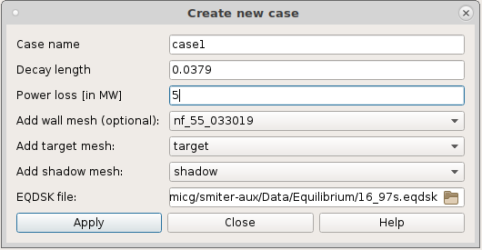
Fig. 2.16 Setting the parameters for the NF55 case.

Equilibrium was shifted outwards the wall mesh, shadow, and target for 25mm. To take that into an account, set beq_rmove (in &beqparameters group) in the control files for all three input meshes:

• wall mesh: beq_rmove = 25 mm
• target: beq_rmove = 25 mm
• shadow: beq_rmove = 25 mm

It is necessary also to determine how to calculate the value of flux for the target at plasma boundary \(\psi_m\) and where to evaluate values of \(R_m\) and \(B_m\) that are being used in the power deposition formula. The only available options are 1 and 9 since these parameters need to be evaluated at the inner midplane.

• target: beq_bdryopt = 9

If the HDSGEN code fails, first check and increase the values of limit_geobj_bin and btree_sizel parameters. In many cases, those two values are responsible for the failure.

Set the POWCAL parameter termination_parameters(1) in the &odesparameter group. This sets the minimum distance (in mm) at which POWCAL avoids any self-intersection incidents and causing the results shown at Fig. 2.4.

• powcal: termination_parameters(1) = 6

Note

Detailed instructions on how to prepare SMITER study are shown in Setting up the case video tutorial.

2.7.4. Results

With both shadow and target mesh ready, move to the Smiter module, create a new case and run it. When the computation completes, open the ParaVis module which allows visualized result analysis.

Note

Detailed instructions on how to use Paraview and display results are available in visualization of power deposition video tutorial.

Fig. 2.17 NF55 benchmark case comparison of the NF55 power deposition, presented in the article [NF55] (Fig. 11(b)), on the left and the power deposition results, obtained by SMITER, on the right.

The final benchmark case results, shown in Fig. 2.17, represent the power deposition scale and wetted area on the target. The maximum power deposition value, obtained by SMITER, is \(q_{peak}=2.206 MW/m^2\) while in the report [NF55] the maximum obtained power deposition value is approximately \(q_{peak}\approx 2.2 MW/m^2\). From that can be concluded that the results, obtained with SMITER, are very similar to the power deposition of FWP4 presented in the PFCFLUX article.

In Fig. 2.18 is shown the wetted NF55 (left) and SMITER (right) case. By splitting the panel to four sub-panels it can be observed that, for the leftmost sub-panel, the yellow peak in both cases occur at around 1200mm.

Fig. 2.18 Comparison of wetted area.

The angle comparison of the same two cases is presented in Fig. 2.19.

Fig. 2.19 Comparison of angles.

Note

In order to compare target mesh with the official 3D CAD model from ITER design office refer to Augumenting results and CAD model in Paraview video tutorial.

2.7.5. Percentage Error

By comparing the angles and \(\psi\) values it can be noticed that they vary a bit from each other.

Differences can be noticed when observing the angles and \(\psi\) values. The PFCFLUX data is stored in the next three files:

• FW4_FACES_2lambdaOpt50mm4mmK4_asymmetric_case26.dat, a file containing node IDs for every 2D triangle cell composing the target mesh.

• FW4_VERTICES_2lambdaOpt50mm4mmK4_asymmetric_case26.dat, a file containing 8 columns with data corresponding to the nodes:

  • Column 1: represents ID of the current node.
  • Column 2: x coordinate of node.
  • Column 3: y coordinate of node.
  • Column 4: z coordinate of node.
  • Column 5: flag for whether a triangle is wetted (value 1) or not (value 0).
  • Column 6: angle at which fieldline hits triangle.
  • Column 7: \(\psi\) values at node.

  Each row corresponds to a single node. Nodes that are listed in this file are the same nodes as those that define the target used in the benchmark study.

• R_Psi_at_ZOMP0d4288m.dat, a file containing \(\psi\) values in correlation to R.

To import scripted data to post-processing tool Paraview, either programmable filter or programmable source can be used. The programmable filter needs to be applied to one of the objects that already exist in the pipeline browser while for the programmable source this is not required. Because each node has its own set of defined values this allows us to, within the ParaView application, to import the required data using the Programmable Filter option.

In order to apply the Programmable Filter first select the benchmark study file in Pipeline Browser. Then, in the menu, navigate to the Filter -> Search, search for Programmable Filter by typing the filter name in the search window and select this option when found. A new dialog will open, containing a scripting window where the python code, which is to be applied to the benchmark study, can be written. In order to import data from previously mentioned files, write the following script.

Note

All PFCFLUX data should be stored to the same directory and the path to this directory can be set with the use of the os.chdir() Python function.

The following example smiter/salome/iter-nf55/programmable-filter-wetted.py inserts two imported fields from PFCFLUX files directly. The remaning are available if Copy Arrays is checked.

# Import libraries
import os
import numpy as np
import vtk
os.chdir(os.path.expanduser("~/smiter/salome/study/iter-nf55/"))
# Read PFCFLUX data
panel='FW4'
shapeType='2lambdaOpt50mm4mmK4_asymmetric_case26'
meshpath=''
vert=np.loadtxt(panel+'_VERTICES_'+shapeType+'.dat')
faces=np.loadtxt(panel+'_FACES_'+shapeType+'.dat').astype(int)
# Define programmable filter arrays
wetted_sum = vtk.vtkDoubleArray()
wetted_sum.SetName("PFCFLUX wetted sum")
wetted = vtk.vtkDoubleArray()
wetted.SetName("PFCFLUX wetted")
for face in range(len(faces)):
    num_wet = (float(vert[faces[face][0]][4])
               + float(vert[faces[face][1]][4])
               + float(vert[faces[face][1]][4]))
    wetted_sum.InsertNextValue(num_wet)
    if num_wet < 2.9 :
        wetted.InsertNextValue(1)
    else:
        wetted.InsertNextValue(0)

out  = self.GetOutput()
out.GetCellData().AddArray(wetted)
out.GetCellData().AddArray(wetted_sum)

2.7.5.1. Angle and \(\psi\) Error

PFCFLUX computes angle values (same goes for \(\psi\)) for each node forming the 2D triangle cell while SMITER computes angle value for each 2D triangle cell (not nodes). In order to get the 2D triangle cell values for the PFCFLUX case, each angle values of the trio-node forming the cell are to be used to calculate the mean angle value.

The angle/\(\psi\) error can then calculated using the next equation:

\(err = 100 \frac{\phi_{pfcflux}-\phi{smiter}}{\phi_{pfcflux}}\)

Following script first calculates the mean value of PFCFLUX angles and \(\psi\) and then the relative error between both results.

# Import libraries
import os
import numpy as np
import vtk
os.chdir(os.path.expanduser("~/smiter/salome/study/iter-nf55/"))
# Read PFCFLUX data
panel='FW4';
shapeType='2lambdaOpt50mm4mmK4_asymmetric_case26';
meshpath='';
vert=np.loadtxt(panel+'_VERTICES_'+shapeType+'.dat');
faces=np.loadtxt(panel+'_FACES_'+shapeType+'.dat').astype(int);
sfac=np.shape(faces);
# Extract PFCFLUX angles and psi values and calculate mean value
pfcfluxangle = []
pfcfluxpsi = []
for face in range(len(faces)):
    indpfcfluxangle = []
    indpfcfluxpsi = []
    for points in range(len(faces[face])):
       indpfcfluxangle.append(vert[faces[face][points]-1][5])
       indpfcfluxpsi.append(vert[faces[face][points]-1][6])
    pfcfluxangle.append(indpfcfluxangle)
    pfcfluxpsi.append(indpfcfluxpsi)
pfcfluxangle = np.array(pfcfluxangle)
pfcflux_ang = []
pfcfluxpsi = np.array(pfcfluxpsi)
pfcflux_psi = []
for i in range(len(pfcfluxangle)):
    pfcflux_ang.append(np.mean(pfcfluxangle[i]))
    pfcflux_psi.append(np.mean(pfcfluxpsi[i]))
pfcflux_ang = np.array(pfcflux_ang)*180/np.pi
# Get data from benchmark study
data = self.GetInput()
smiter_angles = data.GetCellData().GetArray('angle')
smiter_psis = data.GetCellData().GetArray('psista')
# Define programmable filter arrays
out  = self.GetOutput()
ang_error = vtk.vtkDoubleArray()
ang_error.SetName("AnglesError")
psi_error = vtk.vtkDoubleArray()
psi_error.SetName("PsiError")
# Calculate error between angles
for i in range(len(pfcflux_ang)):
    if smiter_angles.GetValue(i) != 0:
       errang = 100*np.abs(pfcflux_ang[i]-smiter_angles.GetValue(i))/pfcflux_ang[i]
       errpsi = 100*np.abs(np.abs(pfcflux_psi[i])-np.abs(smiter_psis.GetValue(i)))/pfcflux_psi[i]
    else:
       errang = 0
       errpsi = 0
    ang_error.InsertNextValue(float(errang))
    psi_error.InsertNextValue(float(errpsi))
out.GetCellData().AddArray(ang_error)
out.GetCellData().AddArray(psi_error)

Note

Note that SMITER does not use angle values directly for the calculation of the power deposition. Instead, it uses dot product between the normal vector and magnetic field vector of the 2D triangle cell.

In the image below we can see percentage error for angles.

Fig. 2.20 Angle comparison of the PFCFLUX and SMITER case. The average observed error is approx. 1.5%. The error, shown by the red area, is greater due to the PFCFLUX returning close to zero power deposition for that area.

Angles in SMITER are calculated from dot product between the normal vector of a triangle and magnetic field vector of 2D triangle cell. Data obtained from the file is directly calculated by PFCFLUX. From the plots displayed in Paraview, we can conclude that the approximate error for \(\psi\) is around 0.01% while for angles is around 1.5%.

Error is larger where surface normal changes faster with position, because we are unable to compare angles at same positions in PFCFLUX and SMITER.

In Fig. 2.21 the percentage error for \(\psi\) values is presented.

Fig. 2.21 Comparison of \(\psi\) values. The error is less than 0.01%.

2.7.5.2. Power Deposition Error

Power deposition is computed using data provided by PFCFLUX. SMITER equation for calculation of power deposition is defined as

\(Q=\frac{FP_{loss}}{2\pi R_m\lambda_mB_{pm}}B.n \exp(-\frac{(\psi-\psi_m)}{\lambda_mRmB_{pm}})\)

while the PFCFLUX power deposition is computed with equation

\(q_{\parallel PFC}=q_{\parallel }(r)R_{omp}/R_{PFC}\)

where \(q_{\parallel }(r)\) is calculated as

\(q_{\parallel }(r)=q_{\parallel omp}\exp(-(r-r_{sep})/\lambda_q)\)

and \(q_{\parallel omp}\) is defined as

\(q_{\parallel omp}=P_{SOL} / (4 \pi R_{omp}\lambda_q (B_{\theta}B_{\Phi})_{omp})\)

The noticed difference between the calculated power depositions, that occur due to the use of different formulas, is approx. 5%, as shown in Fig. 2.22.

Fig. 2.22 Comparison of \(q\) values, with an observed error of approx. 5%.

2.7.6. Plotting output gnuplot files

Modules GEOQ and HDSGEN also produces gnuplot files used for analysing physical quantities (i.e. contour plots of flux gradients). After you have run the case, these gnuplot files can be plotted by simple right clicking on the case in the object browser and click on Plot gnuplot files.

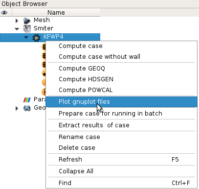
When you click on the Plot gnuplot files a file browser will open that will have a *.gnu filter.

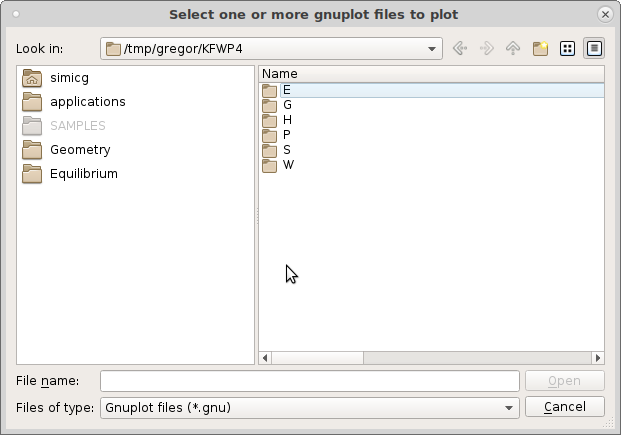
Now enter the /G folder, which houses the GEOQ input and output files for the target mesh.

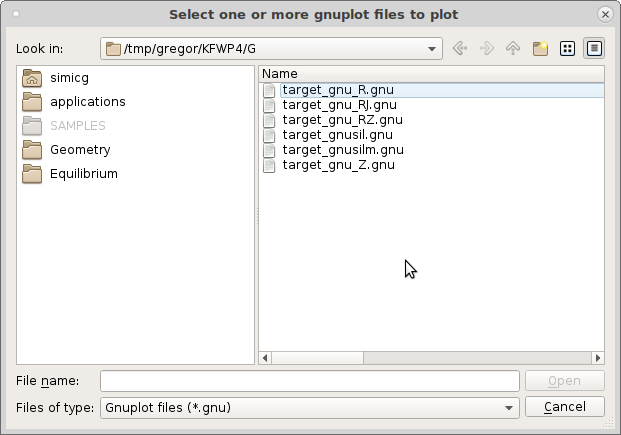
There, select two files, target_gnu_R.gnu and target_gnusil.gnu. To select multiple files, hold the Shift and left click on the files.

Now click Open and the following graph should show up.

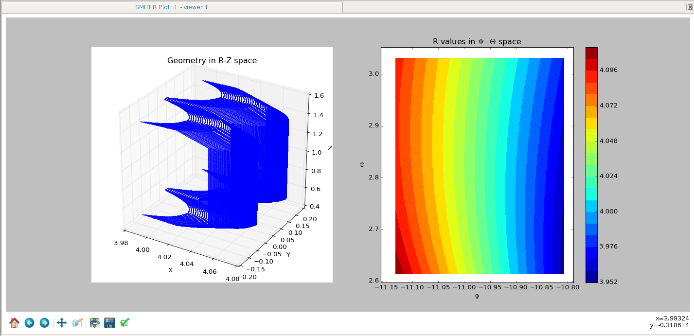
You can plot only one gnuplot file or all in the folder. Each plot is interactive, meaning you can rotate 3D plots and zomm in/out into regions, etc.

Note

Setting plotselections::plot_eqdsk_boundary produce files eqdsk_eqbdry.gnu and eqdsk_eqltr.gnu describing boundary and limiter from eqdsk file.