2.9. Val-vde-botsy-baf (divertor) case¶

This tutorial contains a step-by-step procedure of how to prepare and run the Val-vde-botsy-baf (divertor) case.

2.9.1. Mesh preparation¶

In this subsection will be presented how to prepare meshes for running the case.

For this divertor case, the next three meshes are required:

Wall mesh,

Target mesh and

Shadow mesh

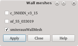
2.9.1.1. Wall mesh¶

Wall mesh is already embedded in SMITER and it can be created by pressing the wallmesh_icon icon. Tick the smiterauxWallMesh and press the Apply button. The mesh will then be added to the MESH module.

../_images/inres1_create_wall_mesh_gui.png

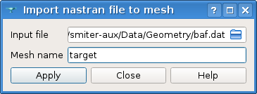
2.9.1.2. Target mesh¶

Use the NASTRAN to MESH tool by clicking on mesh_icon button. Click on the input file browser and proceed to navigate to directory smiter-aux/Data/Geometry/ and select the file named baf.dat. Furthermore, set a name for the new mesh, in this case target, and press Apply.

2.9.1.3. Shadow mesh¶

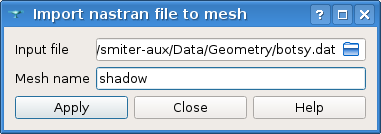
Use the NASTRAN to MESH tool again by either working in the same Nastran to MESH GUI window, opened in the previous Target mesh step, or open a new one by clicking on mesh_icon button. Click on the input file browser and proceed to navigate to directory smiter-aux/Data/Geometry/ and select the file named botsy.dat . Furthermore, set a name for the new mesh, in this case shadow, and press Apply.

2.9.2. Case preparation¶

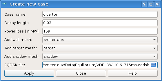
Now go back to the SMITER module. To start a new case, click on the newcase_icon icon found in the SMITER toolbar. A new dialog window will appear on the screen. Here the name of the case, decay length and power loss can be set. Next, choose the wall, target and shadow meshes, created in the previous Mesh preparation step. Finally, add the equilibrium file VDE_DW_li0.6_715ms.eqdsk, found in smiter-aux/Data/Equilibrium/ directory, by selecting it in the file browser. The Decay length in this case is 0.03 m and Power loss is 159 Mw.

List of geometry and equilibrium files used in this study are shown in the table below. Geometry files are found in smiter-aux/Data/Geometry/ and equilibrium files can be found in smiter-aux/Data/Equilibrium/.

Wall mesh	Generated using the tool
Target mesh	baf.dat
Shadow mesh	botsy.dat
Equilibrium file	VDE_DW_li0.6_715ms.eqdsk

After all parameters for this case are set press the Apply button.

Warning

Make sure to close the text dialog when finished setting the parameters, otherwise the changes might not take effect.

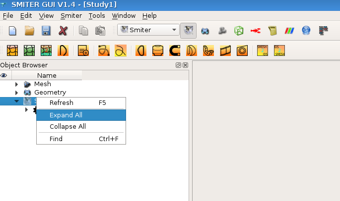
In the Object Browser, by right-clicking on the runsmiter_icon icon and selecting the Expand All option, the full structure of our case will be shown including the geoq, hdsgen and powcal SMITER case objects.

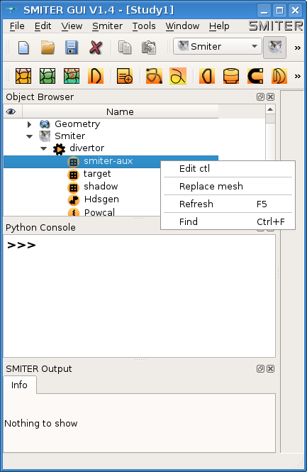
If a change or addition of a specific parameter in the .ctl file is required, right click on mesh and select the Edit ctl option. A dialog window with tabs of group of parameters will open and there the parameter values can be changed if needed.

Warning

Note that you should be familiar with the type of parameter that you want to add or change in order to input it correctly. If the type of input parameter is incorrect, computation will return error. For more information you should check SMITER documentation.

After the required parameters were added or changed, the changes are saved by clicking the Apply button and then closing the dialog window.

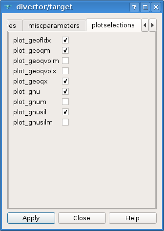
In this tutorial case some of the parameter values in target (baf.ctl) file are needed to be changed. The required changes are listed in the tables below.

Note

The symbol ‘/’ in this tutorials represents the empty parameter value box. For example, if the geoq parameter beq_deltheta had a preset value by default, delete the value and leave the value box empty.

geoq	Default values	target (baf.ctl)
	plotselections	plotselections
	plot_geofldx = .false. plot_gnu = .false. plot_gnum = .true. plot_gnusilm = .true.	plot_geofldx = .true. plot_gnu = .true. plot_gnum = .false. plot_gnusilm = .false.
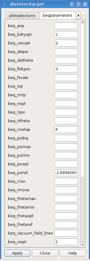
	beqparameters	beqparameters
	beq_cenopt=4 beq_deltheta=0. beq_fldspec=/ beq_nzetap=/ beq_psiopt=2 beq_psieref=PSIREF beq_thetaopt=2 beq_xiopt=/	beq_cenopt=2 beq_deltheta=/ beq_fldspec=3 beq_nzetap=6 beq_psiopt=/ beq_psieref=-2.8968065 beq_thetaopt=/ beq_xiopt=2

The parameter values changes in plotselections:

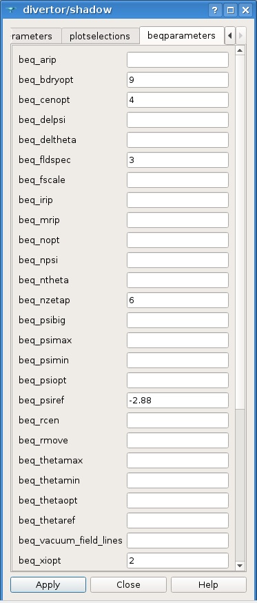
The parameter values changes in bqparameters:

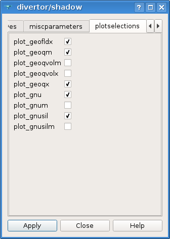
Change of the parameter values is required also in the shadow (botsy.ctl) file.

geoq Default values shadow (botsy.ctl)

plotselections plotselections

plot_geofldx = .false.

plot_gnu = .false.

plot_gnum = .true.

plot_gnusilm = .true.

plot_geofldx = .true.

plot_gnu = .true.

plot_gnum = .false.

plot_gnusilm = .false.

beqparameters beqparameters

beq_bdryopt=5

beq_deltheta=0.

beq_fldspec=/

beq_nzetap=/

beq_psiopt=2

beq_psieref=PSIREF

beq_thetaopt=2

beq_xiopt=/

beq_bdryopt=9

beq_deltheta=/

beq_fldspec=3

beq_nzetap=6

beq_psiopt=/

beq_psieref=-2.88

beq_thetaopt=/

beq_xiopt=2

The parameter values changes in plotselections:

The parameter values changes in bqparameters:

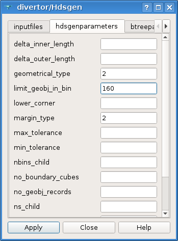
Required parameter changes in the Hdsgen:

Default values Hdsgen (Val-vde-botsy-baf)

hdsgenparameters

limit_geobj_in_bin=20 limit_geobj_in_bin=160

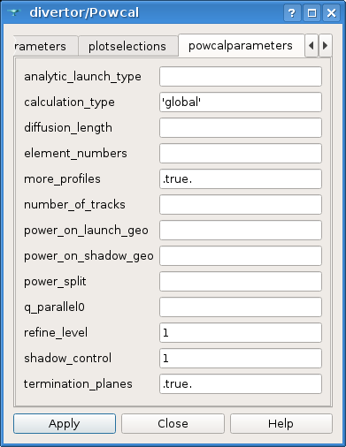
Required parameter changes in the Powcal:

Default values Powcal (Val-vde-botsy-baf)

powcalparameters

calculation_type=’local’

refine_level=/

termination_planes = /

calculation_type=’global’

refine_level=1

termination_planes = .true.

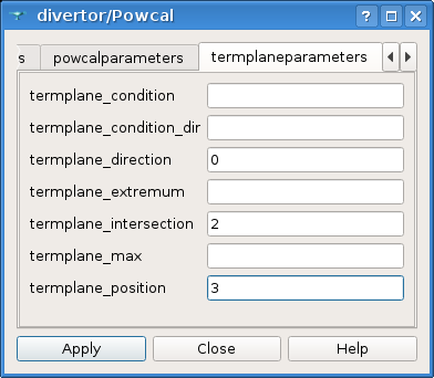
termplaneparameters

termplane_direction=/

termplane_intersection=/

termplane_position=/

termplane_direction=0

termplane_intersection=2

termplane_position=3

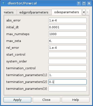
odesparameters

initial_dt=0.01

max_numsteps=/

termination_parameters(1)=/

termination_parameters(2)=/

initial_dt=0.0001

max_numsteps=1000

termination_parameters(1)=1.

termination_parameters(2)=0.1

The parameter values changes in powcalparameters:

The parameter values changes in termplaneparameters:

And at last one, the parameter values changes in odesparameters:

2.9.3. Case computation¶

With the prepared case, the case calculation can be run. That is done by going to the created case case_right_icon icon found in the Object Browser, right clicking on it and selecting the Compute case option.

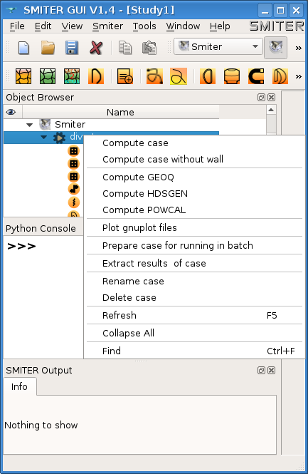
From there the computation will start and the computation process can be observed in the SMITER Output window located below the Object Browser. In it the process of all codes is displayed.

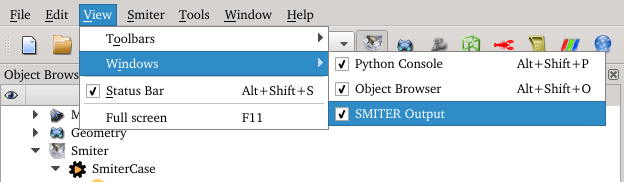
Note

In case the SMITER Output is hidden, activate it by navigating to View -> Windows and then check the SMITER Output option.

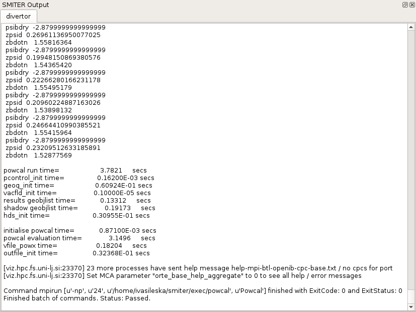
../_images/inres1_smiter_output_tick.png

If the computation is successfully completed, the message Finished batch of commands. Status: Passed. is displayed in the bottom of the SMITER Output window. Furthermore, the PARAVIS module might be auto-opened, displaying the results that are suitable to be viewed with it.

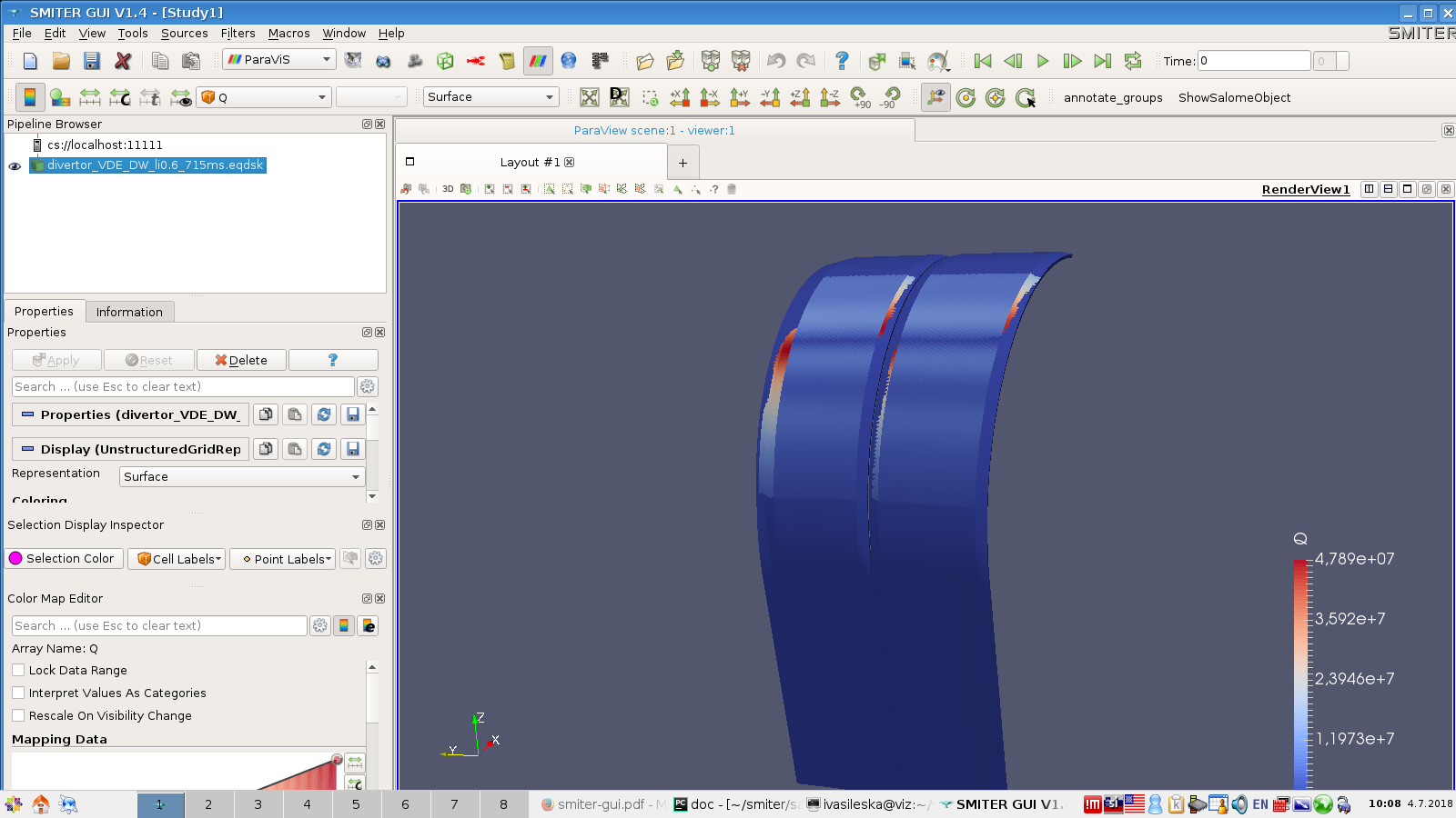
2.9.4. Result analysis¶

2.9.4.1. Power deposition¶

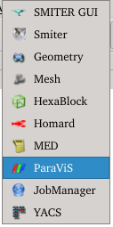
The power deposition results should be automatically displayed in the PARAVIS module after completed computation. In case that this did not occur, activate the PARAVIS module by clicking on the paravis_icon icon in the toolbar or by selecting it from the module list.

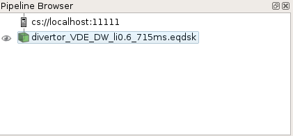
In the Pipeline Browser on the left viewable objects are listed. To view the power deposition results click on the visiblemesh_icon icon and the power deposition results will be displayed in the RenderView window.

Note

The displayed results are actually a VTK file, temporary stored in as /tmp/SmiterCase/P/powcal_pow.vtk. If needed, the file can be manually opened by clicking on the pipeline_icon icon in the Pipeline Browser and then navigating to the mentioned file. The exact path to the powcal_pow.vtk file depends on the name of the case as well as on the working directory.

Note

The ParaVis module is actually complete ParaView tool embedded inside SALOME framework with additional plugins that allow interoperable object referencing (IOR) through CORBA.

Apply button in the Properties panel or click on the visiblemesh_icon icon then shows the result.

Note

A cautionary advice. Whenever you display a VTK file inside ParaViS, it is good to always reset the color scales, if there are any, to the range of the data stored in the VTK.