2.5. Inres1 case
This tutorial contains a step-by-step procedure of how to prepare and run the Inres1 case (see Section 4.3.1 for more details). The step-by-step case preparation procedure starts at subsection Mesh preparation.
For benchmark and testing purposes, an already prepared case is available too and the instructions how to run it can be found in next subsection Running prepared Inres1 case.
2.5.1. Running prepared Inres1 case
This tutorial subsection contains brief instructions on how to open and run
the prepared Inres1 case used as a benchmark case and intended also as a
testing case for SMITER.
The HDF case file can be found in smiter/salome/study/deck/Test-EQ3-inrshad1-inres1.hdf.
If the file is not found then, while in the smiter/salome directory,
fetch the HDF file by running the next command in the terminal:
$ make -C study/deck
To run the case, proceed to open the HDF file by navigating in the menu to
and selecting the HDF file in the file browser.
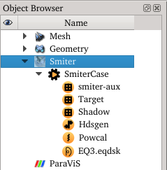
Next, activate the SMITER module, then locate the Smiter tree
found within the Object Browser, expand it, right-click on the
gear icon  of the SMITER case and select the
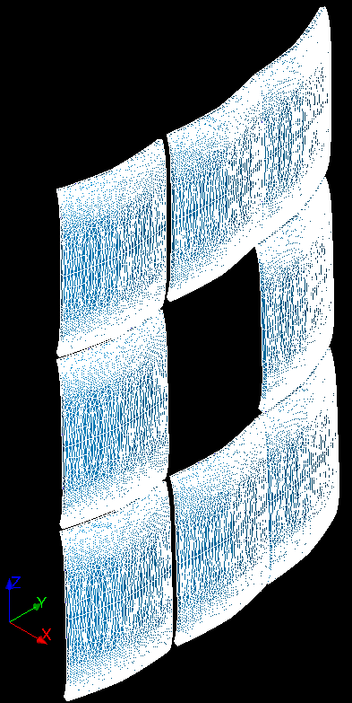
Compute case option. If everything goes well then the results
shown in Fig. 2.1 should appear within a minute.
of the SMITER case and select the
Compute case option. If everything goes well then the results
shown in Fig. 2.1 should appear within a minute.
2.5.2. Mesh preparation
In this subsection will be shown how to prepare meshes for running the case.
Note
An alternative to the manual mesh preparation, using IMAS, is presented in section Importing meshes with IMAS.
For Inres1 case, the next three meshes are required:
- Wall mesh,
- Target mesh and
- Shadow mesh
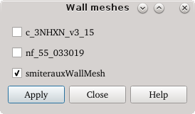
2.5.2.1. Wall mesh
Wall mesh is already embedded in SMITER and it can be created by pressing the
 icon. Tick the smiterauxWallMesh and press
the Apply button. The mesh will then be added to the MESH
module.
icon. Tick the smiterauxWallMesh and press
the Apply button. The mesh will then be added to the MESH
module.
Note
In later stages, after the SMITER case has been created (section
Case preparation), a wall mesh can
also be generated out from the .eqdsk file using
the MESH LIMITER.
Note that the smiterauxWallMesh used in this tutorial and the wall mesh,
generated from the .eqdsk, might be different from each other
(this can easily be checked by displaying the wall meshes
in the MESH module). This will then result in differences
between the obtained calculation results!
2.5.2.2. Target mesh
There are two ways of creating a target mesh for the Inres1 case. First one is to import the STEP format file of the target into the GEOM module and then mesh it in the SMESH module. The second option is to import the NASTRAN file, containing the prepared target mesh, directly into SMITER module. In this tutorial both options will be explored and presented.
2.5.2.2.1. Meshing of target using STEP file
In this subsection the procedure of creating the target mesh from STEP file
format is presented. First it is required to import the STEP file (.stp or
.step) into GEOM module. The STEP file contains Inres1 target CAD
model. Then the meshing procedure is to be done within the SMESH module.
The GEOM module is able to work with many different file formats from
which the CAD models can be imported or either exported from the GEOM
module itself.
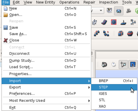
To import the STEP file, move to the GEOM module. This is done by clicking
on icon  in the upper toolbar. Once inside
the GEOM module, navigate to ,
and select
in the upper toolbar. Once inside
the GEOM module, navigate to ,
and select STEP.
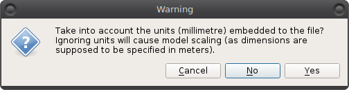
In the opened file browser, navigate to smiter/salome/study/tutorial and select inres1_target.stp. A window will appear, asking if the conversion to meters is required. If option No is selected, the units will be set in milimeters, otherwise the units for the model will be in meters.
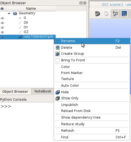
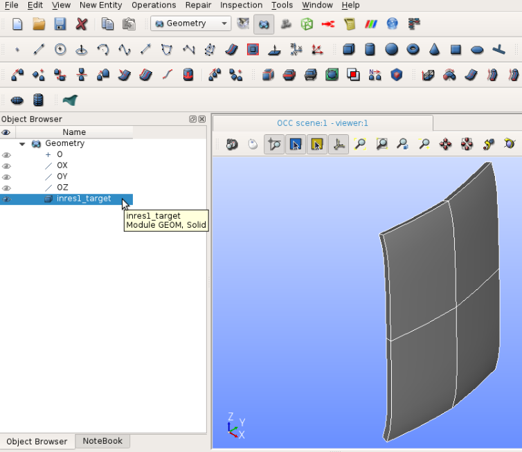
Now move to the Object Browser, where it can be observed that the geometry model, imported from the STEP file, was added to the GEOM module. Here the name of the model can be changed by right clicking on the name in the Object Broswer and setting its name to inres1_target.
Next, move to the SMESH module by clicking on the
 icon. In this module many different operations
can be done, such as translation and rotation of meshes, control
quality of meshes and generation of meshes from CAD models.
icon. In this module many different operations
can be done, such as translation and rotation of meshes, control
quality of meshes and generation of meshes from CAD models.
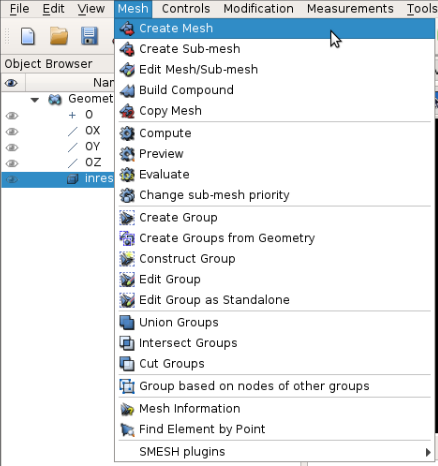
In order create a mesh from a CAD model, a meshing algorithm must first be applied to it. From the top toolbar found in the Smiter window naviage to .
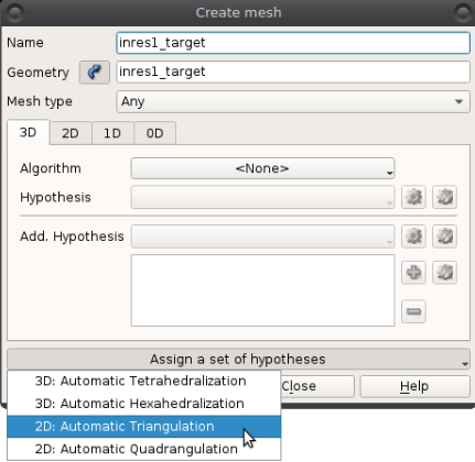
In the popup window, type the name of the new mesh. Then select the geometry object on which the mesh operation is to be done. Select inres1_target found in the Object Browser The name will then be shown in the dialog. For Mesh type there are multiple options that will not be covered in this tutorial. For more information on creating meshes in SMESH module please refer to SMESH Documentation .
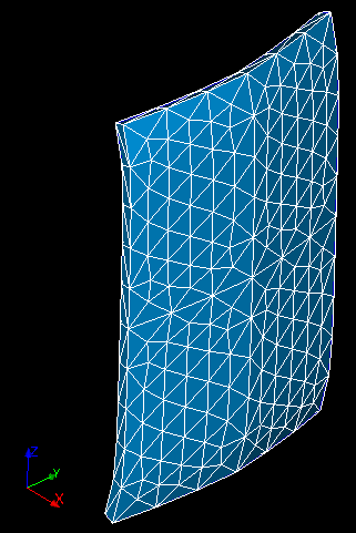
In this tutorial the CAD model will be meshed with triangles that are
are equally distributed in all sections of the model. Click on
Assign a set of hypotheses and select
.
New dialog Hypothesis Construction shows up. Here the name of the
hypothesis can be defined and the maximum length of the triangle edge.
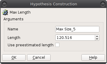
Note
Lower maximum length of the triangle means higher number of triangles. Creation of mesh with higher triangle density means longer computational time.
In this tutorial leave the length as already suggested by Smiter (around 120 mm). Then click the OK button and then the Apply and close button.
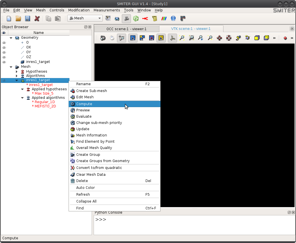
In the Object Browser a new SMESH object was created. By expanding it the hypotheses definition can be seen there. Then right click on the mesh and select Compute. If the computation is successful, the dialog with the mesh informations will pop up. This dialog contains information about number of different types of elements.
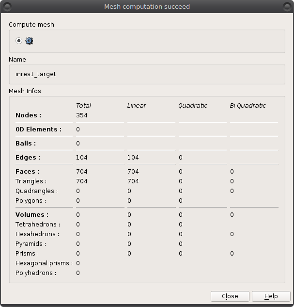
The mesh creation is now completed and it can be used as a target mesh for the SMITER cases.
2.5.2.2.2. Importing the mesh from the NASTRAN file
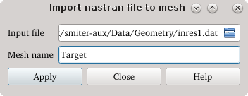
Use the NASTRAN to MESH tool by clicking on  button.
Click on the input file browser and proceed to navigate to directory
button.
Click on the input file browser and proceed to navigate to directory
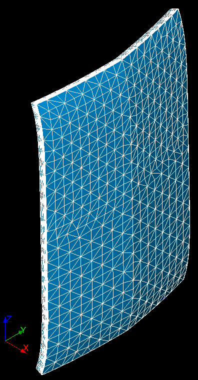
smiter-aux/Data/Geometry/ and select the file named inres1.dat.
Furthermore, set a name for the new mesh, in this case Target, and press
Apply.
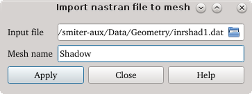
2.5.2.3. Shadow mesh
Use the NASTRAN to MESH tool again by either working in the
same Nastran to MESH GUI window, opened in the previous
Target mesh step,
or open a new one by clicking on button. Click on the input
file browser and proceed to navigate to directory
smiter-aux/Data/Geometry/ and select the file named inrshad1.dat .
Furthermore, set a name for the new mesh, in this case Shadow, and press
Apply.
2.5.3. Case preparation
Note
The procedure how to compute a SMITER case is presented also on the next weblink: https://www.youtube.com/watch?v=ponafnCbm00&list=PLYdrXWbVnKXHzAAfCXw5SDpTDmoKmZFuv&index=3
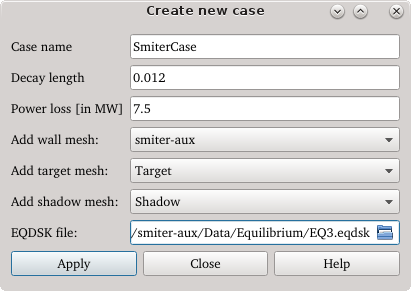
Now go back to the SMITER module. To start a new case, click on the
 icon from SMITER toolbar. A new dialog window will appear
on the screen. Here the name of the case, decay length and power loss can be
set. Next, choose the wall, target and shadow meshes, created in the previous
steps. Finally add the equilibrium file
icon from SMITER toolbar. A new dialog window will appear
on the screen. Here the name of the case, decay length and power loss can be
set. Next, choose the wall, target and shadow meshes, created in the previous
steps. Finally add the equilibrium file EQ3.eqdsk, found in
smiter-aux/Data/Equilibrium/ directory, by selecting it in the file browser.
List of geometry and equilibrium files used in this study are shown
below. Geometry files are found in smiter-aux/Data/Geometry/ and
equilibrium files can be found in smiter-aux/Data/Equilibrium/.
| Wall mesh | Generated using the tool |
| Target mesh | inres1.dat |
| Shadow mesh | inrshad1.dat |
| Equilibrium file | EQ3.eqdsk |
After the required parameters were added or changed, the changes are saved by clicking the Apply button and then closing the dialog window.
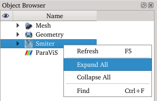
In the Object Browser, by right-clicking on the
 icon and selecting the Expand All option,
the full structure of our case will be shown including the
icon and selecting the Expand All option,
the full structure of our case will be shown including the geoq, hdsgen
and powcal SMITER case objects.
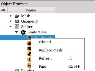
If a change or addition of a specific parameter in the .ctl file is
required, right click on mesh and select the Edit ctl option.
A dialog window with tabs of group of parameters will
open and there the parameter values can be changed.
For inres1 case the following parameters must be changed:
smiter-aux:
beq_cenopt: 4beq_bdryopt: 3beq_deltheta: 0.beq_rmove: -6
target:
plot_geoqx: [x]plot_geoqm: [x]plot_gnum: [x]plot_gnusil: [x]plot_gnusilm: [x]beq_cenopt: 4beq_psiopt: 2beq_thetaopt: 2beq_deltheta: 0.beq_rmove: -6beq_psiref: PSIREF
shadow:
plot_geoqx: [x]plot_geoqm: [x]plot_gnum: [x]plot_gnusil: [x]plot_gnusilm: [x]beq_cenopt: 4beq_psiopt: 2beq_bdryopt: 5beq_thetaopt: 2beq_deltheta: 0.beq_rmove: -6beq_psiref: PSIREF
Hdsgen:
limit_geobj_in_bin: 20geometrical_type: 2margin_type: 2tree_nxyz: 1,2,2tree_ttalg: 2tree_type: 3position_tranform: 1plot_hdsm: [x]plot_hdsq: [x]plot_geobjq: [x]plot_geoptq: [x]
Powcal:
plot_powx: [x],calculation_type: ‘local’power_loss: 7.5e+06shadow_control: 1more_profiles: .true.rel_error: 1.e-4abs_error: 1.e-4initial_dt: 0.01max_zeta: 6.
Warning
Note that you should be familiar with the type of parameter that you want to add or change in order to input it correctly. If the type of input parameter is incorrect, computation will return error. For more information you should check SMITER documentation.
After the required parameters are set, press the Apply button and then close the dialog window.
2.5.4. Case computation
With the case prepared, the case calculation can be run. That is done by
going to the created case icon found in the
Object Browser, right clicking on it and selecting
the Compute case option.
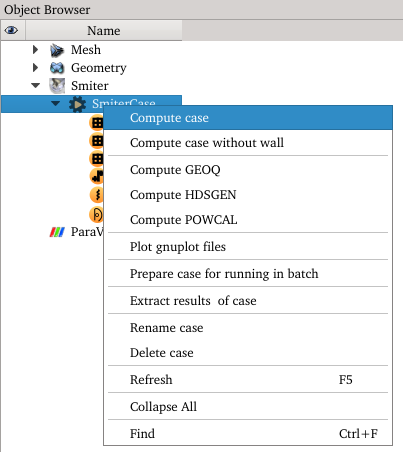
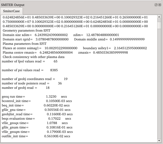
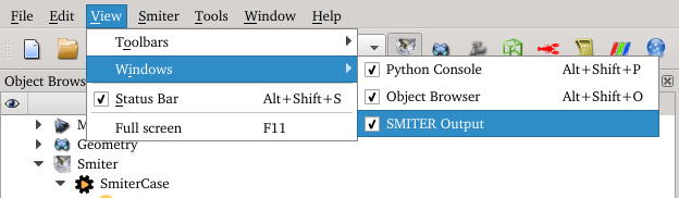
From there the computation will start and the computation process can be observed in the SMITER Output window located below the Object Browser. In it the process of all codes is displayed.
Note
In case the SMITER Output is hidden, activate it by navigating to View -> Windows and then check the SMITER Output option.
If the computation is successfully completed, the message
Finished batch of commands. Status: Passed. is displayed in the bottom of
the SMITER Output window. Furthermore, the PARAVIS
module might be auto-opened, displaying the results that are suitable
to be viewed with it.
2.5.5. Result analysis
2.5.5.1. Power deposition
The power deposition results should be automatically displayed in the
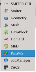
ParaViS module after completed computation. In case that this
did not occur, activate the PARAVIS module by clicking on the
 icon in the toolbar or by selecting it from the
module list.
icon in the toolbar or by selecting it from the
module list.
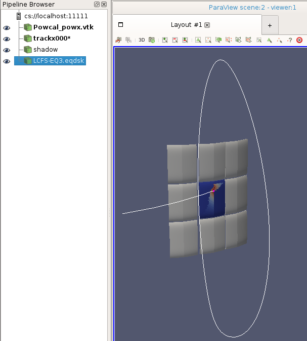
In the Pipeline Browser on the left viewable objects are listed.
To view the power deposition results click on the ![]() icon
and the power deposition results will be displayed in the
RenderView window.
icon
and the power deposition results will be displayed in the
RenderView window.
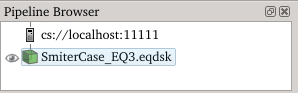
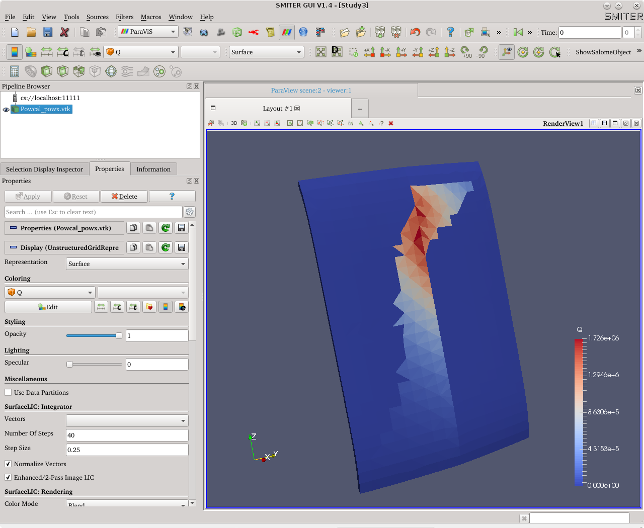
Fig. 2.1 Inres1 results in ParaViS module
Note
The displayed results are actually a VTK file, temporary stored in
as /tmp/SmiterCase/P/powcal_pow.vtk. If needed, the file can be
manually opened by clicking on the  icon in the
Pipeline Browser and then navigating to the mentioned file.
The exact path to the
icon in the
Pipeline Browser and then navigating to the mentioned file.
The exact path to the powcal_pow.vtk file depends on the name of
the case as well as on the working directory.
Note
The module is actually complete ParaView tool embedded inside SALOME framework with additional plugins that allow interoperable object referencing (IOR) through CORBA.
Note
A cautionary advice. Whenever you display a VTK file inside ParaViS, it is good to always reset the color scales, if there are any, to the range of the data stored in the VTK.
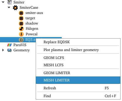
2.5.5.2. Plotting the plasma flux contour
The steps to view the plot of the plasma flux contour are:
- Open Smiter module
- Navigate to the Object Browser
- Expand the SMITER case object tree (either by right clicking on the
icon and selecting Expand All or clicking on
the tree arrow besides the icon)
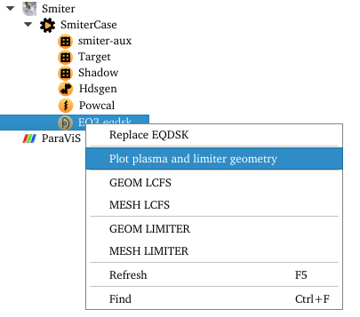
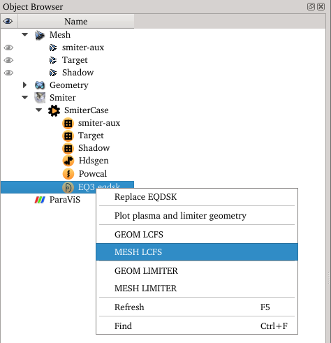
- Right click on the
.eqdskobject, marked with icon
icon - Select the Plot plasma and limiter geometry option.
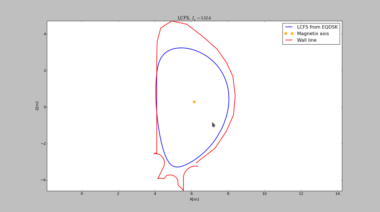
Then the plasma flux contour plot will be shown in the Viewer window.
Note
The plot of the plasma flux contour is created from the loaded
.eqdsk file and using Python plotting library matplotlib.
2.5.6. Fieldline tracing
In this subsection the preparation procedure of the fieldline tracing for this case and the procedure of displaying the results will be presented.
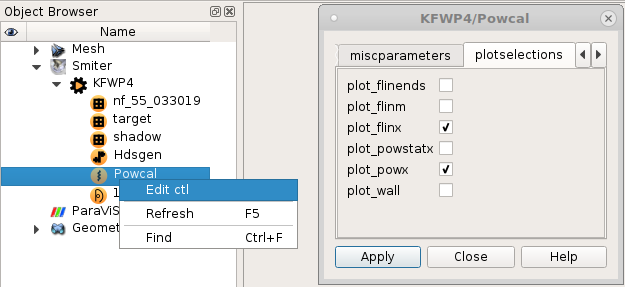
2.5.6.1. Edit and recompute Powcal
First the Powcal of this SMITER case needs to be edited and recomputed.
Powcal can be edited by right clicking on its name found in the SMITER
case object tree and selecting edit .ctl. Next, in the opened window select
plotselection tab, check the plot_flinx 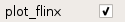 option
and press Apply.
option
and press Apply.
Note
For larger cases, when multiple fieldlines need to be collected, the plugin described in Save fieldlines to HDF5 can be used.
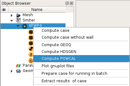
The Powcal is now ready to be recomputed. To recompute only the Powcal,
right click on the SMITER case icon and select
the Compute POWCAL option.
2.5.6.2. Cell selection on the target
After the Powcal computation is finished, activate the ParaViS
module .
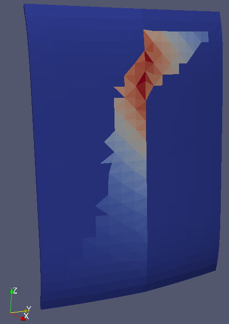
A new object will be shown in the Pipeline Browser, representing
the target with corresponding Q values to the mesh elements. Turn on the display
of this object by clicking the ![]() icon left of the object
label. The mesh and corresponding values will be shown in the
RenderView window.
icon left of the object
label. The mesh and corresponding values will be shown in the
RenderView window.
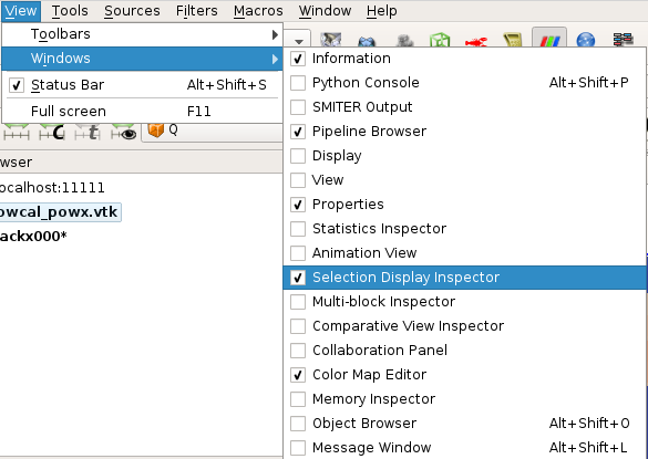
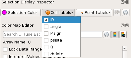
Next, check if the Selection Display Inspector is shown on the
left side in the ParaViS window. If it is hidden, it can be shown by
navigating in the top menu bar
View -> Windows submenu and checking the
Selection Display Inspector  .
.
With the Selection Display Inspector shown, turn on the ID box in the Cell Labels list. This will now allow us see the the ID of the mesh element in the next step.
Next, select a triangle cell in the mesh for which you want to get the fieldline.
That can done by using the tools on the the Render View menu
 , either Select cells on
  (also S
keyboard button) or Interactive Select Cells On
(also S
keyboard button) or Interactive Select Cells On
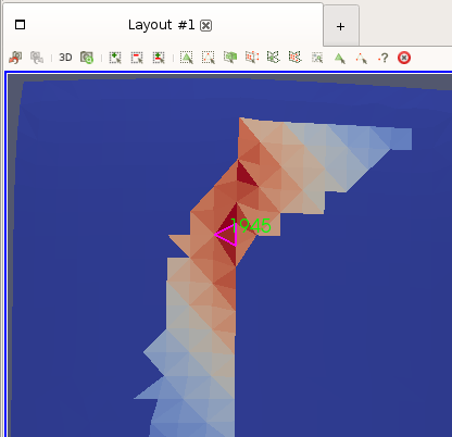
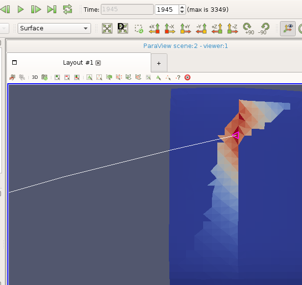
 Select the triangle as shown in the following figure. In this tutorial the cell
with the ID
Select the triangle as shown in the following figure. In this tutorial the cell
with the ID 1945 was selected.
2.5.6.3. Set fieldline trace
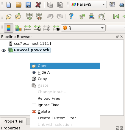
Next, the files containing fieldline traces are required to be opened in
ParaVis module. This is done by right clicking on the
icon in the Pipeline Browser and
selecting Open option.
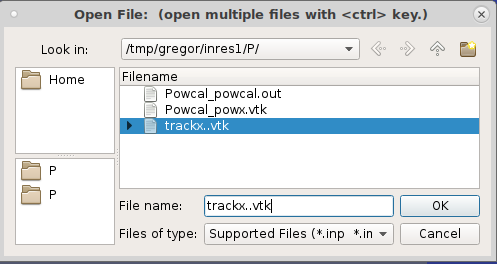
Proceed to navigate to files located in /tmp/{SMITER_case_name}/P,
select the trackx.vtk file (it is actually a set of files) and press
OK.
A new object named trackx000* will be shown
Pipeline Browser.
In the Time control entry 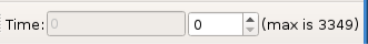 , located on the right upper corner of
the
, located on the right upper corner of
the ParaViS window, insert the ID of the triangle, in this case
1945, and press Enter.
Then proceed to set on the visibility of the trackx000* in
Pipeline Browser and the fieldline trace for the selected cell
will be shown in the ParaVis Render View window.
2.5.6.4. Set the remaining meshes
2.5.6.4.1. Shadow
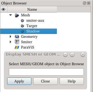
To show the shadow in ParaView, activate the Smiter module and
click on the Show MESH/GEOM in ParaView  dialog. Select
and highlight the shadow mesh, found in the
dialog. Select
and highlight the shadow mesh, found in the
Object Browser under the Mesh object tree,
and click on Apply on the dialog. If the dialog doesn’t close by
itself, press the Close button.
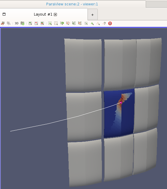
Now the shadow mesh too will be available in ParaVis. Head back to the
ParaVis module and turn on the display of the shadow.
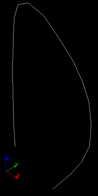
2.5.6.4.2. LCFS
The obtained fieldline traces are correct if they end on the LCFS. To check
that, first go back to the
module, right click on EQ3.eqdsk and select
option. This will create the LCFS mesh.
Next, the same as for the shadow mesh, click on
Show MESH/GEOM in ParaView , highlight the
LCFS-EQ3.eqdsk mesh object and click Apply
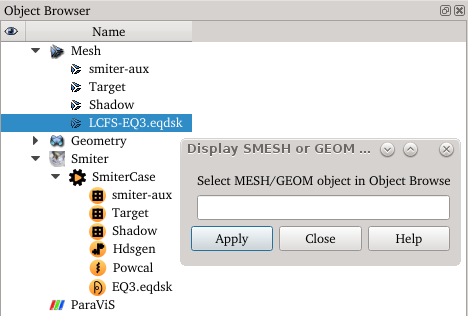
Now the LCFS geometry will also be displayed in ParaView. Click on
.
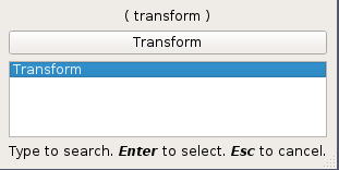
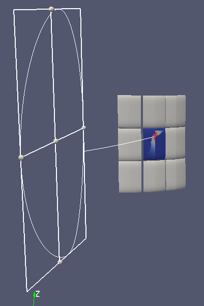
Next, the LCFS needs to be rotated and translated to the right place in order
to see if the fieldline trace ens in OMP. Press Ctrl and
space on the keyboard. In the searchbox type Transform
and press enter.
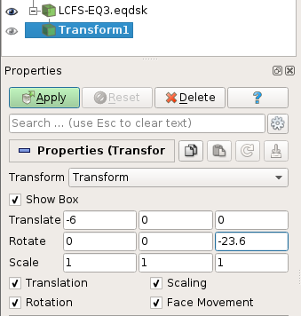
A new property panel Transform will be shown. Here the Rotate,
Translate and Scale parameters can be set. Set the Rotate angle
value around the Z axis (third field from the left) to -23.6. Then set
the Translate in the X axis value (first field from the left) to -6.
While inserting the transform values, the Show box in the Render View
window, which serves as a preview for the new position of the limiter geometry,
will be instantly updated. When finished press the Apply button.
The transformed LCFS by the default name Transform1 will be created in the
Pipeline Browser.
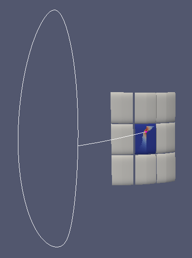
To run off the Show box, unmark the Show Box option of the translated
LCFS in the Properties section. Now it can be observed that the
end of fieldline tracing is correct.
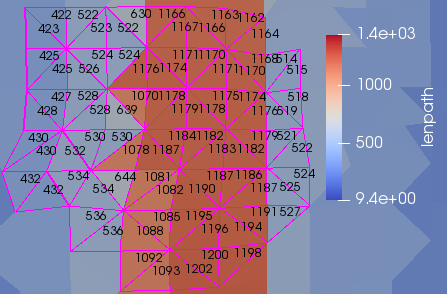
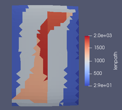
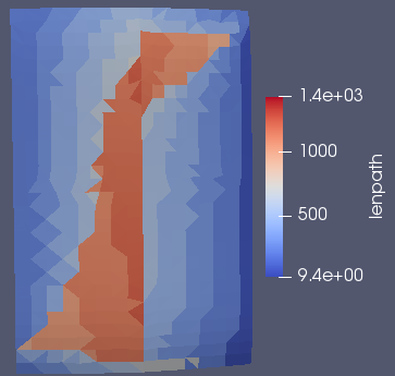
2.5.6.5. Connection length
Connection length is calculated in variable lenpath available in
ParaViS module by selecting Coloring in
Properties where we get the following result:
For increased accuracy we change the Powcal parameters in
Object Browser within activated SMITER module by
right-click on Powcal and selecting Edit ctl. Under
odesparameters we set abs_error and
rel_error to 1e-6 and then with right-click on inres1
case Compute POWCAL to get new results for ParaViS.
To see the lengths on selected triangles we enable and then
Cell Labels check lenpath to be displayed. Then in
RenderView1 we press key s to select single cell or use
other cell selections modes to select multiple cells. By prescribing
Cell Label Format to %.0f and color to black in
Selection Label Properties we can get the following display.