2.3. Meshing CAD models¶

In this tutorial we will create meshes for SMITER from surface CAD models extracted beforehand. Unless we continue from Extracting FW4 CAD surface tutorial we need to ensure that study files are available for reading with

make -C study/tutorial

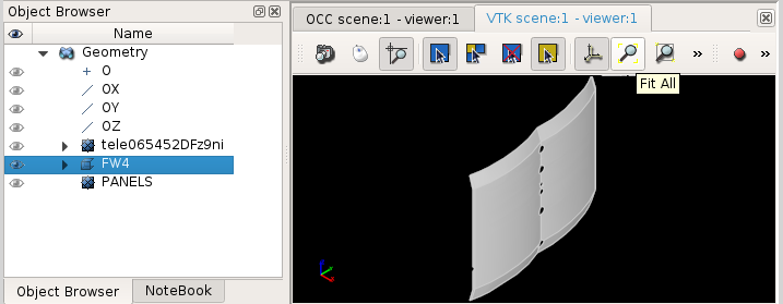
We open study/mesh1.hdf study that contains CAD geometry with FW4 and PANELS from which we will create target and shadow meshes. Before we go to meshing we activate the Geometry module with a click on icon_geometry_module button from the toolbar. We setup visibility of both models by clicking on icon_visiblemesh icons and Fit All to get ready for meshing.

Mesh for the target is usually required to be higher density that the shadow as we want better wetted pattern on the target. It is always good practice to find the correct mesh density by firstly trying rough meshes that are still acceptable from past experience and then doubling the density by recomputing the meshes.

2.3.1. Meshing FW4¶

Now we can move to Mesh module by clicking icon_mesh_module in the main toolbar. While being in Mesh module we again select FW4 geometry and set visibility by icon_visiblemesh and Fit All and the FW4 panel appears in the Mesh module.

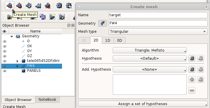
From the menu we select Mesh ‣ Create mesh or icon_mesh_init button the meshing toolbar where we setup dialog with the Name to target and Mesh type to Triangular. For Algorithm we select Triangle: Mefisto as shown in the following image.

Before pressing Apply and Close we click on Assign a set of hypotesses and within Hypothesis Construction dialog change Name to Max Size Target and Length to 20. This will create Hypothesis for Wire discretisation Algorithm in 1D tab.

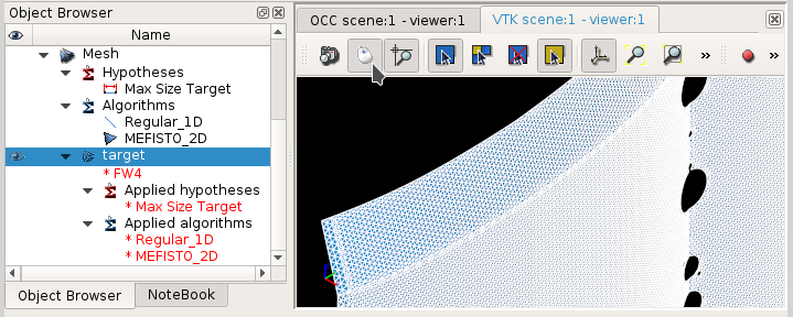
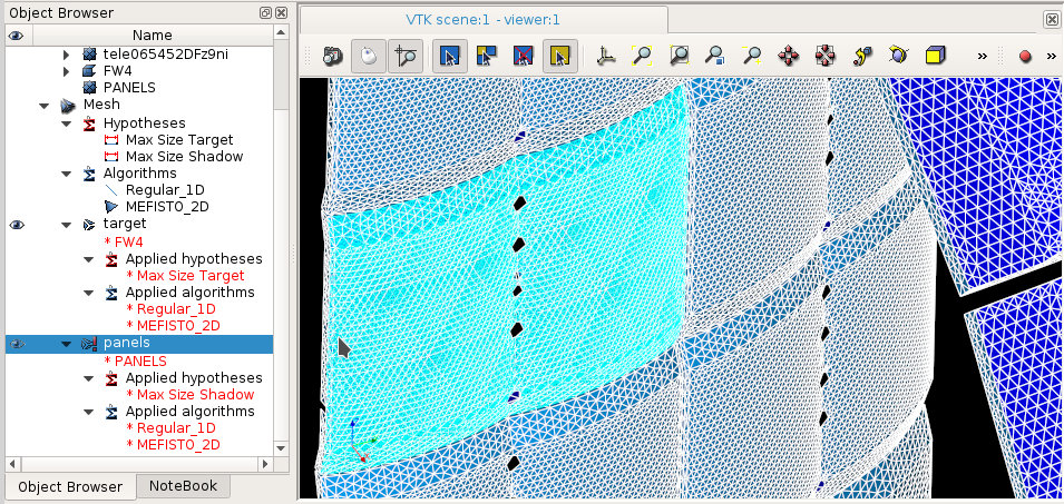
At Apply and Close and Mesh ‣ Compute from the menu or icon_mesh_compute button from the meshing toolbar we get newly created mesh statistics stating 18545 triangles created ifor the target mesh. After Close and inpecting Object Browser and zooming mesh we obtain the follwoing image.

2.3.2. Creating shadow mesh¶

For creating the panels mesh we again Mesh ‣ Create mesh or icon_mesh_init with PANELS selected from the Geometry. The only difference is that we Assign a set of hypotheses for 2D: Automatic Triangulation with Max Size Shadow Name and Length set to 50 that created arounf 165000 triangles shadow mesh with some errors in shape evaluation that seems OK.

We will now create rotated panels with menu selection Modification ‣ Transformation ‣ Rotation, where we Select whole mesh… named panels. Rotation axis and point of rotation needs to be entered as shown in the folowing image.

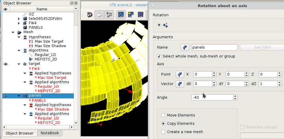
With Preview enabled we Copy Elements with Angle -40 degrees of rotation that gets created in the study after Apply and Close.

2.3.3. Translating target¶

In order to avoid intersection of the target with the shadow panels due do different meshing density and numerical errors we translate the target panel by less that 0.01 mm inwards. From menu Modification ‣ Transformation ‣ Translation we open a dialog for translation. The relative translation vector can be easily determined by firstly clicking on the center of the panel in “two-point” mode and then dividing that point position by 1000 or so to get small translation in the correct direction inwards.

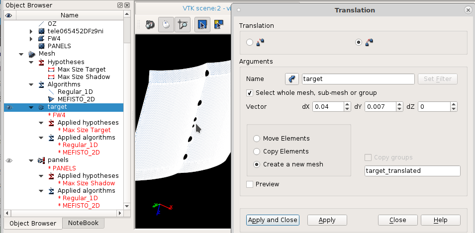
With this operation we have now prepared all meshes necessary to compute the case and can save the study somewhere. Mesh panels will serve as a shadow and target_translated will be a target for SMITER.

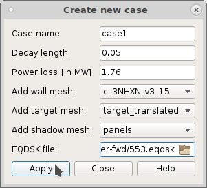
2.4. Computing the case¶

In this tutorial we will create SMITER case with meshes prepared in Meshing CAD models tutorial. Unless we continue from Meshing CAD models tutorial we need to ensure that study files are available for reading with

make -C smiter/salome/study/tutorial

We open study/mesh2.hdf study that contains first wall CAD geometry with corresponding target and shadow meshes.

We change the following beqparameters in associated Eqdsk meshes by right clicking on them and selecting Edit ctl to:

beq_bdryopt=9

Required for limiter case. We set this for meshes shadow and target.

beq_fldspec=3

Mapping equilibrium field to cylindrical (axisymmetric). Set for meshes wall, shadow and target.

beq_bdryopt=3

Set this for wall mesh LIMITER-554.eqdsk. It calculates the value of flux at plasma boundary while also including the wall silhouette.

beq_nzetap=1

Set for shadow and target.

For hierarhical data structure (HDS) we need to increase “bin size” Hdsgen CTL hdsgenparameters

limit_geoobj_in_bin=200

Default value was 20 objects (triangles).

See Val-F11-fw246t-fw4t for similar test case parameters or press Help button when setting parameters.

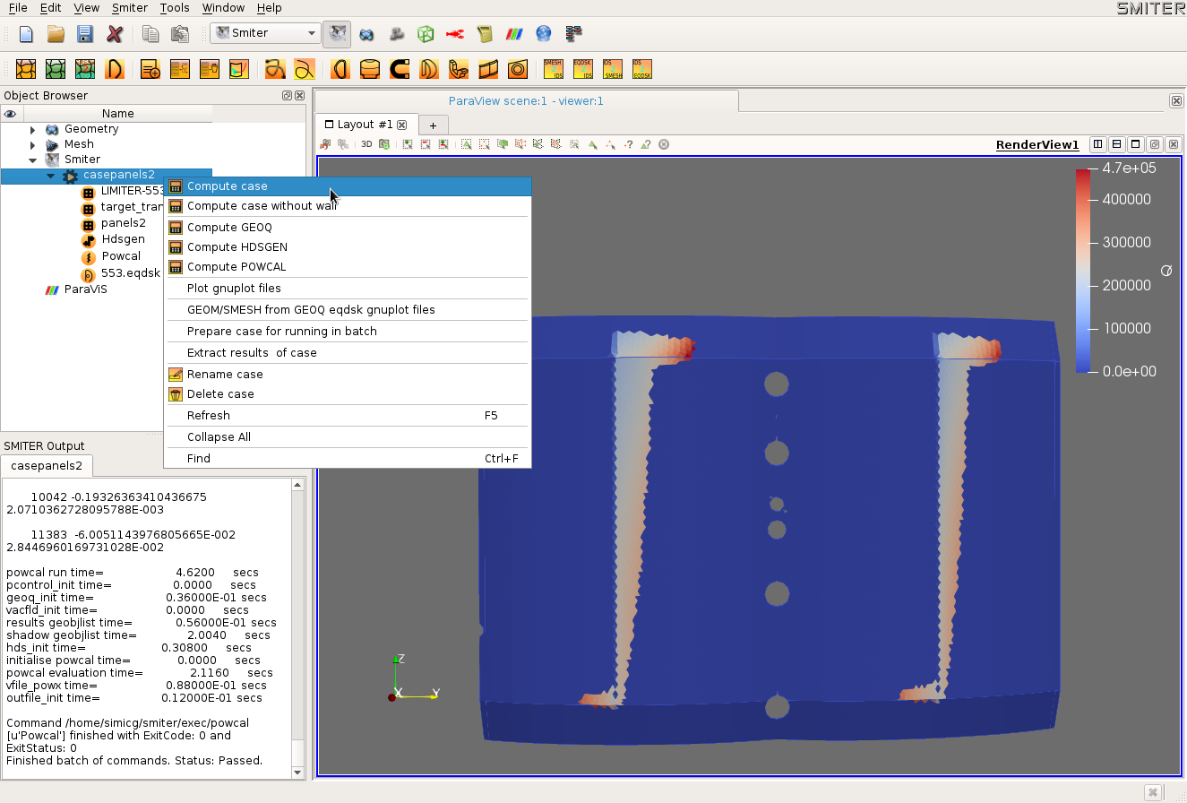
After right clicking on Compute case the following results appear automatically.

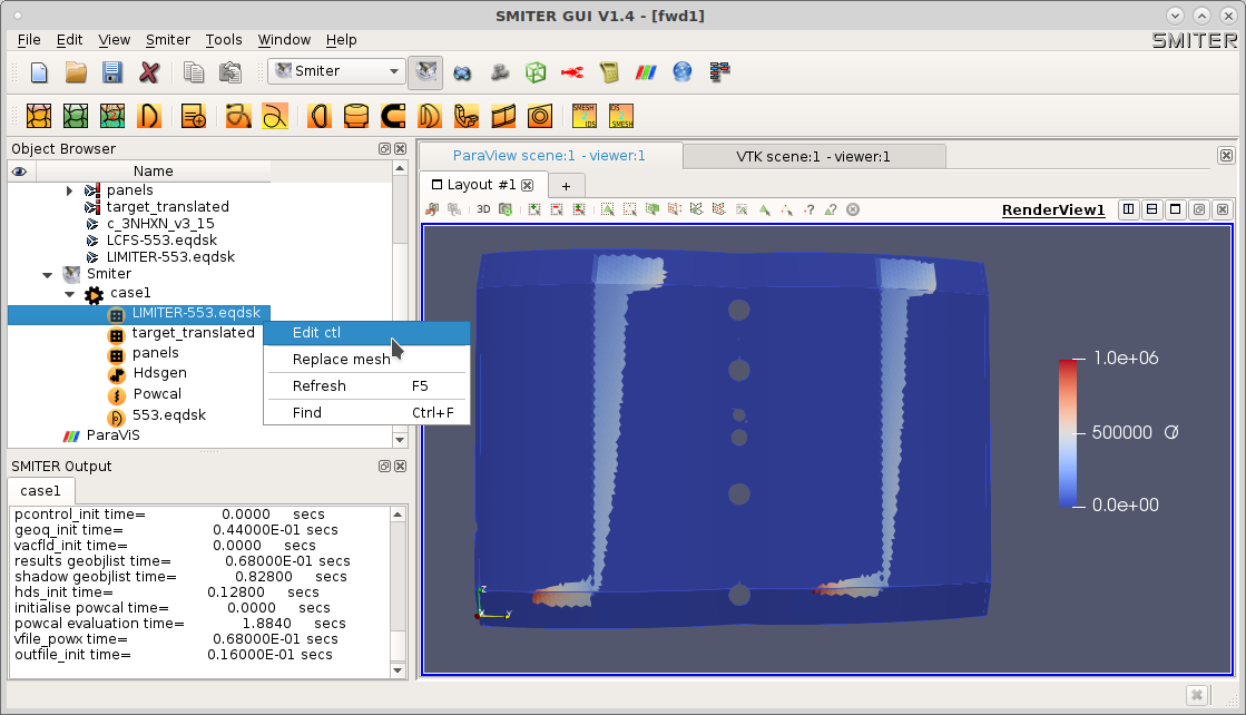
When comparing the wetted pattern with NF55 benchmark case we see similarity in the shape. Maximal heat flux should be proportional to power loss \(1.76 MW/ 7.5 MW \cdot 2.2 MW/m^2=0.52 MW/m^2\), while here we observe \(Q_{max}=1.0 MW/m^2\)

The study is available as study/tutorial/fwd1.hdf.

The difference is due to small shadow. If we increase the shadow by rotating left and dight we get \(Q_{max}=0.47\) which is close to the estimation and available as study/tutorial/fwd2.hdf and shown in the following figure.