3.1. Background¶

Heat always moves from area with higher temperature to the area with lower temperature. Amount of heat, going through an area of size \(A\), is defined as

(3.1)¶\[Q = k\frac{A(T_a-T_b)t}{d}\]

where k is the heat conductivity of the area, that heat passes through, d is the width of the area, A is the cross-section of the area, t is time and \(T_a\) and \(T_b\) are temperatures on each side of the surface. Here we can derive heat flux that is defined as power per area.

(3.2)¶\[q =\frac{Q}{At} = k\frac{(T_a-T_b)t}{d}\]

In Fig. 3.1 is an example of simple heat transfer model.

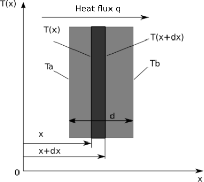
Fig. 3.1 Scheme of simple heat transfer model.

For the model along x-axis one can write general equation

(3.3)¶\[q = \frac{T(x)-T(x+\triangle x)}{\triangle x}= -\frac{T(x+\triangle x)-T(x)}{\triangle x}\]

Or for infinitely small step one can say

(3.4)¶\[q=q(x)=-k\frac{d T(x)}{d x}\]

Equation above presents Fourier’s law of heat transfer, that can be defined in three-dimensional space.

(3.5)¶\[q(r,t)= -k\nabla T(r,t)\]

This equation has the following components

(3.6)¶\[q_x = -k_x\frac{\partial T(x,y,z,t)}{\partial x}\]

(3.7)¶\[q_y = -k_y\frac{\partial T(x,y,z,t)}{\partial y}\]

(3.8)¶\[q_z = -k_z\frac{\partial T(x,y,z,t)}{\partial z}\]

Where \(k_x\), \(k_y\) and \(k_z\) are heat condictivities in x, y and z axes. The heat conductivities of isotropic materials are equal in all directions \(k=k_x=k_y=k_z\). Result of all three components is equal to

(3.9)¶\[q(x,y,z,t) = \sqrt{q_x^2+q_y^2+q_z^2}\]

3.1.1. Heat Transfer in Solids¶

Solid is defined in cartesian coordinate system. There are two main types of thermal loading. Heat fluxes on the body are \(q1,q2,q3\), etc. Inside the body there is heat source \(Q(x,y,z)\). Due to thermal loading the temperature distribution of the body changes. One can write it as \(T(x,y,z)\). Equation of heat transfer is derived from Fourier’s law of heat transfer and law of energy conservation.

(3.10)¶\[-\left(\frac{\partial q_x}{\partial x}+\frac{\partial q_y}{\partial y}+\frac{\partial q_z}{\partial z}\right)+Q=\rho c\frac{\partial T}{\partial t}\]

If we include the definition of heat fluxes in the upper equation, we get

(3.11)¶\[\begin{split}\frac{\partial}{\partial x} \left(k\frac{\partial T(x,y,z,t)}{\partial x}\right)+\frac{\partial}{\partial y}\left(k\frac{\partial T(x,y,z,t)}{\partial y}\right)+\frac{\partial}{\partial y}\left(k\frac{\partial T(x,y,z,t)}{\partial z}\right) \\ +Q(x,y,z,t)=\rho c\frac{\partial T(x,y,z,t)}{\partial t}\end{split}\]

Upper equation defines the heat transfer of solid bodies, where \(\rho\) is density of the body and c is specific heat of the material of body. Time-independent heat transfer is defined as

(3.12)¶\[\begin{split}\frac{\partial}{\partial x}\left(k\frac{\partial T(x,y,z,t)}{\partial x}\right)+\frac{\partial}{\partial y}\left(k\frac{\partial T(x,y,z,t)}{\partial y}\right)+\frac{\partial}{\partial y}\left(k\frac{\partial T(x,y,z,t)}{\partial z}\right) \\ +Q(x,y,z,t)=0\end{split}\]

Boundary conditions are

Temperature on the surface \(S_1\):

(3.13)¶\[T_s=T_1(x,y,z,t)\]

Heat flux on the surface \(S_2\):

(3.14)¶\[q_xn_x+q_zn_z+q_zn_z=-q_s\]

Fluid temperature and heat transfer coefficient on the surface \(S_3\):

(3.15)¶\[q_xn_x+q_zn_z+q_zn_z =h(T_s-T_f)\]

3.1.2. Finite Element Method Formulation¶

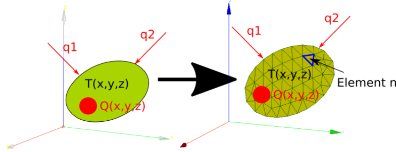
Fig. 3.2 Left: Analytical heat transfer model. Right: Finite element heat transfer model.

The solution of a finite element heat transfer model is temperature in the nodes of the mesh. Frist we have to prepare the mesh. Then we can define interpolation functions for every finite element \(\psi (x,y,z)\). Interpolation functions have three rules:

The number of monomials is equal to the number of nodes in an element.

Interpolation functions must guarantee continuous field of primary variable (temperature) accross the edges of finite element. Same goes for their derivative (heat flux).

Monomials of individual interpolation function are independent of each other.

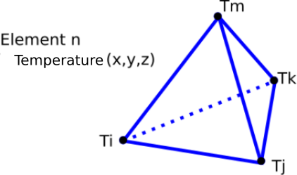
Fig. 3.3 Example of tetrahedron.

Interpolation function of meshes with tetrahedron is defined as

(3.16)¶\[\psi(x,y,z)=C_11+C_2x+C_3y+C_4z\]

Every node in the tetrahedron has its own interpolation function. Each interpolation function \(\psi_i\) has the following values in the nodes of the element with coordinates \((x_i,y_i,z_i)\).

(3.17)¶\[\begin{split}\psi_i(x_i,y_i,z_i) = \begin{cases} 1 & \quad j = i\\ 0 & \quad j \neq i \end{cases} i,j = 1,..,N\end{split}\]

Sum of all interpolation functions in an element must be equal to 1. This guarantees that primary variable (temperature) across the field of the element can be constant.

(3.18)¶\[\displaystyle\sum_{j=1}^{N} \psi_j(x,y,z) = 1\]

Temperature gradients in the element can be expressed as

(3.19)¶\[\begin{split}\begin{Bmatrix} \dfrac{\partial T(x,y,z,t)}{\partial x} \\[2.5ex] \dfrac{\partial T(x,y,z,t)}{\partial y} \\[2.5ex] \dfrac{\partial T(x,y,z,t)}{\partial z} \end{Bmatrix} = \begin{bmatrix} \dfrac{\partial \psi_i}{\partial x} \dfrac{\partial \psi_j}{\partial x} \dfrac{\partial \psi_m}{\partial x} \dfrac{\partial \psi_k}{\partial x}\\[2.5ex] \dfrac{\partial \psi_i}{\partial y} \dfrac{\partial \psi_j}{\partial y} \dfrac{\partial \psi_m}{\partial y} \dfrac{\partial \psi_k}{\partial y} \\[2.5ex] \dfrac{\partial \psi_i}{\partial z} \dfrac{\partial \psi_j}{\partial z} \dfrac{\partial \psi_m}{\partial z} \dfrac{\partial \psi_k}{\partial z} \end{bmatrix} {T}=[B]{T}\end{split}\]

3.1.3. Galerkin Method¶

Galerkin method (named after russian mathematician Boris Galerkin) is the method of determining the weight function of a differential equation. Galerkin method suggests that weight functions should be equal to the interpolation functions of the finite element. Differential equation of physical problem is \(D(\phi)\) for volume of \(\text{V}\). Boundary condition of the differential equation is \(B(\phi)\) on the surface \(\text{S}\). Mathematical model is defined as

(3.20)¶\[\int_V W_1D(\phi)\mathrm{d}v + \int_V W_2B(\phi)\mathrm{d}s = 0\]

Weight functions in the upper equation are \(W_1\) and \(W_2\). The model is then discretized in small subesctions called finite elements. Thus we get approximate solution with differential equation \(D(\psi(r)\phi)\) for finite element volume of \(\text{V}\) and boundary condition \(B(\psi(r)\phi)\) on the edge of finite element. Approximate model can be expressed as

(3.21)¶\[\int_V W_{1j}D(\sum\psi_i(r)\phi_i)\mathrm{d}v + \int_S W_{2j}B(\sum\psi_i(r)\phi_i)\mathrm{d}s=R\]

Weight functions in the upper equation are again \(W_1\) and \(W_2\). Galerkin method suggests that weight functions are equal to interpolation functions of finite element. It also suggests that \(R -> 0\), which leads to \(W_{1j}=\psi(r)\) and \(W_{2j}=\psi(r)\). With the Galerkin method we can write the general equation of heat transfer

(3.22)¶\[\int_V\left( \frac{\partial q_x}{x}+\frac{\partial q_y}{y}+\frac{\partial q_z}{z} \right)\psi_i\mathrm{d}v=0\]

If we include boundary conditions in the upper equation, we get finite element equations with heat flux and temperature distribution in the nodes of the element.

(3.23)¶\[\begin{split}\int_V \rho c \frac{\partial T(x,y,z,t)}{\partial t}\phi_i\mathrm{d}v-\int_V\left(\frac{\partial \psi_i}{\partial x}\frac{ \partial \psi_i}{\partial y} \frac{\partial \psi_i}{\partial z}\right){q}\mathrm{d}v = \\ \int_v Q\psi_i\mathrm{d}v-\int_{s1}{q}^T{n}\psi_i\mathrm{d}s- \int_{s2}q_s\psi_i\mathrm{d}s-\int_{s3}h(T-T_f)\psi_i\mathrm{d}s\end{split}\]

The heat flux on the surface is \({q}^T={q_x q_y q_z}\) and normal vector on the surface \({n}^T={n_x n_y n_z}\). Temperature distribution can be expressed as

(3.24)¶\[[C]{\dot(T)}+({K_c}+[K_h]){T}={R_t}+{R_q}+{R_h}\]

In the upper equation the coefficient matrices are

Heat capacity matrix \([C]\):

(3.25)¶\[[C]=\int_v \rho c [N]^T[N]\mathrm{d}v\]

Heat conduction matrix \([K_c]\):

(3.26)¶\[[K_c]=\int_v k [B]^T[B]\mathrm{d}v\]

Heat convection matrix \([K_h]\):

(3.27)¶\[[K_h]=\int_{S3} h [N]^T[N]\mathrm{d}s\]

Node values are given as

Temperature on surface \(S_1\):

(3.28)¶\[{R_T}=-\int_{S_1}{q}^T{n}[N]^T\mathrm{d}s\]

Heat source of body:

(3.29)¶\[{R_Q}=\int_vQ[N]^T\mathrm{d}v\]

Heat flux on surface \(S_2\):

(3.30)¶\[{R_q}=\int_{S2} q_s[N]^T\mathrm{d}s\]

Convection heat flux on surface \(S_3\):

(3.31)¶\[{R_h}=\int_{S3}hT_f[N]^T\mathrm{d}s\]

3.2. ITER First Wall thermal model¶

Scheme of temperature case preparation is shown in the figure Fig. 3.4.

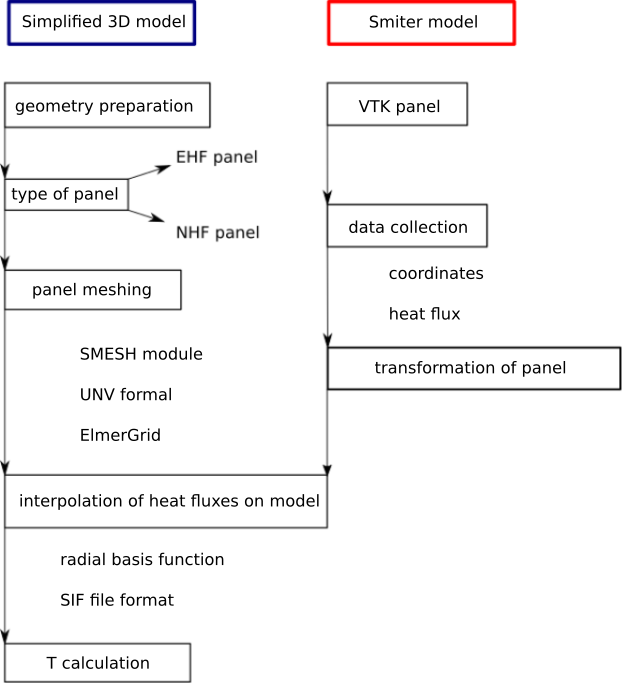
Fig. 3.4 Computation scheme of the temperature case.

Temperature study can be split in the following sections:

Geometry preparation: The code must prepare the appropriate geometry of a simplified finger model according to the chosen type of the panel. There are two different types of fingers, one for EHF panel and the other for NHF panel. Geometry is prepared in GEOM module, which is a module for preparation of CAD models and is included into SMITER GUI. GEOM module includes Python libraries that can be used for scripting of geometry.

Panel meshing: When the geometry is prepared, we can mesh it. Meshing algorithms used in the code are part of SMESH module, which is a meshing module in SMITER GUI. SMESH module comes with Python libraries that were used to mesh the finger model. After the model is meshed, we first export it to universal file format (.unv), which is further converted to elmer mesh files (.mesh.), that are used in the study.

Smiter panel definition: Here the user must choose the appropriate vtk file that contains triangular mesh of the panel and power deposition values, calculated in SMITER module. User must also define the position of panel in the poloidal direction. This position defines angle of inclination, that is later used when we align the panel with the simplified model of fingers. The position of panel in poloidal direction also defines the type of panel (EHF or NHF).

Transformation of panel: After we read the data from appropriate vtk file, we must translate the nodes so that they overlap with the simplified model of fingers. This is needed so that we can later easily map the heat fluxes from one surface to another.

Interpolation of heat fluxes: After the surfaces overlap or are at least aligned, we can map the heat fluxes from SMITER vtk panel onto simplified model of fingers. The mapping function is radial basis function and is part of Python’s scientific package scipy.

Temperature calculation: When the heat fluxes are mapped, we can define all boundary conditions on the simplified model. Boundary conditions are stored into special file with .sif extension, that contains alld the data of the simplified finger model and is read by the Elmer program, which then calculates the temperatures.

The chosen vtk panel must be translated is space so that it overlaps with the simplified model of finger. Ideally, both surfaces would completely overlap. This way the mapping of heat fluxes would be very accurate. In reality, this is difficult to achieve, beacuse different panels have different toroidal curvature of the plasma facing surface. Also different panels with different surfaces are tested all the time, so the appropriate approximation was needed. Heat flux is mapped with the help of radial basis function. EHF panel has 40 fingers (20 on the left and 20 on the right side). Individual fingers and the computations of each finger are completely independent of each other. The only thing that changes is the plasma heat flux on the surface. This means that we get output vtk file with result for every panel. A script was written which reads all those 40 vtk files and stores the data into one vtk file with all the fingers.

3.2.1. Mesh files¶

Open source FEM package Elmer FEM contains multiple source codes, that combine the solving of problems with finite element method. Command ElmerGrid reads mesh, that can be defined in multiple formats and can be converted into another format. Some of the possible input formats are Abaqus CAE input format .inp and Ansys input format ansys. Since SMESM module od SMITER GUI, where we are preparing the meshes for temperature calculation, allows us to export meshes in unv universal file format and this same format is also input format for ElmerGrid, we can just use unv format to convert our meshes to appropriate Elmer mesh. Second argument of the command ElmerGrid is the format of output mesh. The command ElmerSolver needs special type of mesh with .mesh. keyword. In Linux terminal the command would look like

ElmerGrid 8 2 nameOfFile.unv

After the command is executed we get the following files:

mesh.boundary

mesh.elements

mesh.header

mesh.names

mesh.nodes

3.2.1.1. File mesh.header¶

File mesh.header contains number of nodes and elements in the mesh. Example is presented below. In the first line we have number of nodes, number of elements and number of elements on the edges. The second line contains the number, that tells us the number of different elements defined in the mesh. Next lines contain type of individual element and number of those elements.

In the example above one can see that the mesh has 300 nodes, 261 elements and 76 elements, that are defined on the edges of the mesh. There are two different types of elements in the mesh. Mesh has 261 elements with the type 404 (four-nodes finite element) and 76 elements with the type 202 (line with two nodes).

3.2.1.2. File mesh.node¶

File mesh.node contains identification numbers and coordinates of nodes. Every line starts with two numbers of type integer. Those two numbers define the ID number of node and the parallel index of node. Elmer skips the parallel index if we do not compute the program with parallel settings. Last three numbers are of type float and present the coordinates of the node x, y and z, as shown below.

n1 p x y z
n2 p x y z
...
nn p x y z

3.2.1.3. File mesh.element¶

This file contains element data. Every lines starts with a number of type integer. This number defines the ID number of element. Next number defines the number of body that this element is assigned to. This is followed by the type of finite element, and finally the ID numbers of nodes, assigned to the element.

e1 telo tip n1 ... nn
e2 telo tip n1 ... nn
...
en telo tip n1 ... nn

3.2.1.4. File mesh.boundary¶

File mesh.boundary contains data on elements that are part of the boundary region. First number in line is the ID number of element, followed by the ID number of boundary region, where this element is defined. Boundary regions have their own ID number and are specified according to different boundary conditions defined on the model. Element can be defined in multiple boundary regions. Next value presents the type of element, followed by the ID numbers of nodes.

e1 rob p1 p2 type n1 ... nn
e2 rob p1 p2 type n1 ... nn
...
en rob p1 p2 type n1 ... nn

3.2.2. File SIF¶

After we converted the unv file to Elmer mesh files, we can specify the boundary conditions, material properties and other parameters that influence the calculation of temperatures. We specify those parametersr in a special file with sif extension. Structure of the sif file has many sections.

Header

Simulation

Constants

Body n

Material n

Body Force n

Equation n

Solver n

Boundary Condition n

Initial Condition n

Component n

Letter n presents the number of individual section, that defines individual boundary condition or material, etc. Through those different numebrs the program can differ between different boundary conditions, material properties, etc.

3.2.2.2. Simulation¶

In this section one has to define parameters that define the modelling of partial differential equations that need to be solved in order to compute temperatures correctly. Here one can define the steady-state or transient system, coordinate system and output files. Below is the example of Simulation section of EHF panel.

Simulation
Max Output Level = 5
Coordinate System = Cartesian
Coordinate Mapping(3) = 1 2 3
Simulation Type = Steady state
Steady State Max Iterations = 1
Output Intervals = 1
Timestepping Method = BDF
BDF Order = 1
Solver Input File = case.sif
Post File = case.vtu
End

3.2.2.3. Constants¶

In this section one can define constants used in the study. Example is shown below.

Constants
Gravity(4) = 0 -1 0 9.82
Stefan Boltzmann = 5.67e-08
End

3.2.2.4. Body and Material Definition¶

Elmer mesh files contain also information on different body and boundary regions where different boundary conditions are defined. Booundary conditions and material properties can be temperature dependent. We can write this dependency in the sif file in the tabular form. For more complex boundary condition and material properties definitions we can write user defined functions in Fortran90. Below is the definition of heat conductivity of beryllium shield on the EHF panel.

Material 1
Name = "Beryllium"
Heat Conductivity = Variable Temperature
Real
20   200
100  169
200  144
300  127
400  116
500  107
600  100
700  91
End
End

Definition of material properties depends on the physical model that we are calculating.

3.2.2.5. Equation and Solver Definition¶

In this section one can define the solver according to out physical model. With the solver we define the model that we want to solve. We can define multiple solvers if we want to process different physical phenomena. For every solver we can define the number of iterations, convergence tolerance, etc. With solver we can also define different output files and properties that we want to post-process. Below is the example of solver that solves heat transfer model for EHF panel.

Solver 1
Equation = Heat Equation
Procedure = "HeatSolve" "HeatSolver"
Variable 1 = Temperature
Exec Solver = Always
Stabilize = True
Bubbles = False
Lumped Mass Matrix = False
Optimize Bandwidth = True
Steady State Convergence Tolerance = 1.0e-10
Nonlinear System Convergence Tolerance = 1.0e-20
Nonlinear System Max Iterations = 20
Nonlinear System Newton After Iterations = 3
Nonlinear System Newton After Tolerance = 1.0e-20
Nonlinear System Relaxation Factor = 0.2
Linear System Solver = Direct
Linear System Direct Method = Banded
End

3.2.2.6. Boundary Condition Definition¶

In this chapter one defines the boundary conditions of the model. Elmer mesh files define ID numbers of different bodies and boundary regions that have their own unique ID number. This ID numbers are used in sif files for boundary conditions.

Boundary Condition 1
Target Boundaries(1) = 11
Name = "adiabaticBC"
Heat Flux = 0.001
End

Above is an example of adiabatic boundary condition for EHF panel. In the first line there is the ID number of boundary condition. Second line contains ID numbers of target boundaries. There can be multiple target boundaries. Second line gives the name of the boundary condition. Following lines contain actual definition of boundary condition.

3.2.3. Model Preparation¶

3.2.3.1. Enhanced Heat Flux Panel¶

Enhanced heat flux panel is a panel that can sustain thermal loadings up to \(4.7MW/m^2\). It is an axisymmetric panel with 20 fingers on each side. Component, located on top of the finger is known as hypervapotron. Hypervaptron is constructed of two cooling tanks, that are connected with each other at the end of the finger. This tank system is responsible for the cooling of the finger. Hypervapotron can generally be divided into two different corss-sections, that are shown in figure Fig. 3.5. In the left side on the figure there is a channel where water enters the fingers and the beam itself. Channels of hypervapotron and the tank are joined together at the end of the finger, as mentioned previously. On the right side one can see the cross-section without the bottom tank. In Elmer module the simplified mesh consists only of one cross-section. In ITER reactor there are 176 EHF panels, that will be produced and supplied by Russian Federation. Provided Abaqus CAE study defines the constant heat flux of \(350000\text{W/m}^\text{2}\) on the whole panel, except for small quadratic area on the panel where peak heat flux of \(4700000\text{W/m}^\text{2}\) is studied. This thermal loading will never appear in a real-case scenario. The purpose of this study was to show reaction of fingers to such high loading.

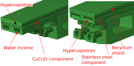
Fig. 3.5 In the left side on the figure there is a channel where water enters the fingers and the beam itself. Channels of hypervapotron and the tank are joined together at the end of the finger, as mentioned previously. On the right side one can see the cross-section without the bottom tank.

The important part of the Elmer module is geometry preparation. The plasma facing side of the model should resemble the original structure as much as possible. Because of that we have to focus on hypervapotron. Cross-section and parameters are shown in figure Fig. 3.6.

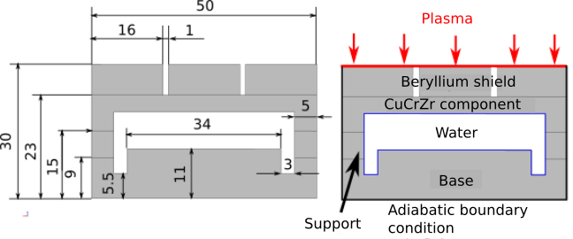
Fig. 3.6 In the left side there are dimensions of the EHF simplified cross-section model. In the right side there are defined boundary conditions and names of components.

On top of the panel there are three subcomponents. First component, exposed to plasma is beryllium shield. Under beryllium shield there is component of CuCrZr. Bottom components are named support and base and are made of stainless steel with label SS316. Between those components is a water channel. Dimensions of each component are shown in figure Fig. 3.6. The program that generates the cross-section, was written in Python programming language with the help of GEOM module. Based on the given geometry the program first deifnes vertices, then edges, faces and finally solids. In GEOM module we can define all basic geometry entities, that help us build the CAD model. First we have to load the proper libraries. We do that with the following script

# Study initialisation
salome.salome_init()
# GEOM library import
import GEOM
# geomBuilder import
from salome.geom import geomBuilder
# Definition of geomy object of class geomBuilder
geompy = geomBuilder.New()

In the program we defined the geompy object of class geomBuilder, that enables us to define different geometrical objects inside GEOM module. This object contains methods like MakeVertex, MakeEdge, MakeFace and many others that help us define complex objects in GEOM module. Steps of geometry preparation are given below:

Vertex definition: First we have to define vertices that defien our model. We do that with method MakeVertex.

# Vertices definition for first wire model
pt1 = geompy.MakeVertex(0,0,0)
pt2 = geompy.MakeVertex(0,10,0)
pt3 = geompy.MakeVertex(10,10,0)
pt4 = geompy.MakeVertex(10,0,0)
# Vertices definition for second wire model
pt5 = geompy.MakeVertex(2,2,0)
pt6 = geompy.MakeVertex(2,8,0)
pt7 = geompy.MakeVertex(8,8,0)
pt8 = geompy.MakeVertex(8,2,0)

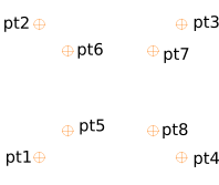
Fig. 3.7 Definition of vertices in GEOM module.

Edges definition: Now one has to connect vertices into edges. Edges can be straight lines or an arc of circle and other curves. This way our model is defined in 2D surface because there is an area that is limited by those edges. We do that with the method MakeEdge.

# Edge definition for first wire model
e1 = geompy.MakeEdge(pt1,pt2)
e2 = geompy.MakeEdge(pt2,pt3)
e3 = geompy.MakeEdge(pt3,pt4)
e4 = geompy.MakeEdge(pt4,pt1)
# Edge definition for second wire model
e5 = geompy.MakeEdge(pt5,pt6)
e6 = geompy.MakeEdge(pt6,pt7)
e7 = geompy.MakeEdge(pt7,pt8)
e8 = geompy.MakeEdge(pt8,pt5)

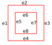
Fig. 3.8 Definition of edges in GEOM module.

Face model definition: When the wire model is defined and encloses a particular area, we can fill that particular area and create a surface model. Surface model is defined with method MakeFace that takes one closed wire model as input argument and with method MakeFaceWires that takes two wire models as input arguments and creates a face between those two wire models.

# Transformation of wire models into face model
compound = geompy.MakeFaceWires([w1,w2])

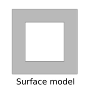
Fig. 3.9 Definition of face model in GEOM module.

Partition model definition: To partition a model we have to divide the exsting face model into more face submodels that together form a previous full face model. Those face submodels all define different properties of a full model (for example boundary conditions or material properties). There are two ways to define face submodels. We can define them in the beginning and then join them into one full model. Second way to do that is to first define full face model and then divide (partition) it into smaller subsections. GEOM method used for that purpose is MakePartition. In Elmer code the full model is divided into submodels. Example is shown in code below.

# Definition of edge that will partition the model
e_partition = geompy.MakeEdge(pt1,pt3)
# Partition of the model
partition = geompy.MakePartition([compound],[e_partition])

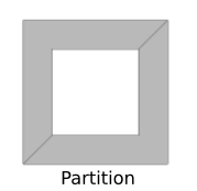
Fig. 3.10 Example of face partition in GEOM module.

Now that the cross-section of model is finished, it needs to be extruded into 3D space to get the 3D model of the finger. First we have to define the etrusion curve. Along this curve we will extrude the cross-section. this curve defines curvature of panel in the toroidal direction. Points for creation of the curve were extracted from the Abaqus study, provided by ITER organisation. Points on the top right edge of the beryllium shield were stored into text file and then imported into Python. Then they were stored into array. Then the curve was defined with method MakeInterpol. The curve was translated so that the right top point of the cross section was coincide with the first point of the curve. Tangent of the curve in this point must be perpendicular to the cross-section. Then we extrude cross-section in space along thiss curve. This way we get the full 3D model of the finger. Then the model needs to be meshed. To do this, one must use a proper meshing algorithms. Mesh module of SMITER enivronment enables us to mesh geometric models. First, the proper SMESH libraries needs to be imported into Python.

# Salome library import
import salome
# Initialisation of Salome program
salome.salome_init()
# smeshBuilder library import
from salome.smesh import smeshBuilder
# Definition of smeshBuilder object
smesh = smeshBuilder.New()

The final result of meshing is the unstructured grid of tetrahedrons. For every dimension one must define the proper approximate size of tetrahedrons.

# Definition of mesh based on selected geometry
tetramesh = smesh.Mesh(geometry, "geometry")
# Definition of 1D algorithm
algo1D = tetramesh.Segment()
# Definition of approximate length of edges of tetrahedrons
algo1D.LocalLength(1.0/100.0)
# Definition of 2D algorithm
algo2D = tetramesh.Triangle()
algo2D.LengthFromEdges()
# Definition of 3D algorithm
algo3D = tetramesh.Tetrahedron()
# Mesh computation
ret = tetramesh.Compute()

First one must define the geometry that needs to be meshed. Then the algorithm for meshing must be defined. Many types of different algorithms existinside Mesh module that can be used for meshing of CAD models. One can define multiple hypotheses like number of segments, length of edges, etc. Approximate length of edges is defined in Elmer code. This means that after mesh computation the approximate length of edges will be the same as the one that we defined on the Python script. The basis for hypotheses in two- and three-dimensional space come from the edge length definition. The computation of those mesh elements like triangles and tetrahedrons is based on the one-dimensional hypotheses. During the meshing process, the subsections like beryllium shield, CuCrZr component, support and base are taken into an account as well. The mesh is then converted into unv mesh type and then into ElmerGrid mesh.

3.2.3.2. Normal Heat Flux Panel¶

Normal heat flux panel is the other type of panel (first being EHF panel) of first wall in ITER tokamak. The maximum power deposition on this panel is \(2\text{MW/m}^\text{2}\). Just like EHF panel then NHF panel is axisymmetric and is built of fingers, that are attached to the beam or base of the panel, that is further attached to the other components. Those fingers have different cross-section than EHF fingers. The full NHF structure is shown in figure \(NHF_hypervapotron_fullStructure\). On top of the panel is beryllium shield, that carries the biggest thermal loading on the surface. Under the shield there is CuC1 support and the CuCrZr support, that contains two water channels. Both channels are wrapped with stainless steel pipes. Width of the wrapping component is 1 mm. The problem of this small wrapping components is that one has to increase the mesh density in order to avoid meshing problems in this part of the model. Due to simplifying the model and calculation time of high-density meshes one has to consider whether it is useful to increase the density of mesh. The stainless steel pipe is therefore excluded, since its influence on the final result is small. Below CuCrZr structure there is stainless steel base, attached to the beam. Altogether there is 215 NHF panels int tokamak. They were developed and produced by the European Union. There is 13 different types of NHF panels. They differ in length, width and number of fingers, depending on their location in the tokamak. The cross-sectioon of fingers does not change. The cross-section is shown on figure \(NHF_panelCrossSection\). Procedure for CAD modelling and mesh preparation is the same as in EHF panel. CAD model was prepared in GEOM module. Mesh was prepared in mesh module.

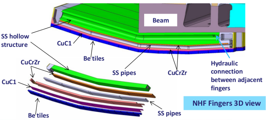
../_images/NHF_hypervapotron_fullStructure.png

Fig. 3.11 Full structure of NHF panel.

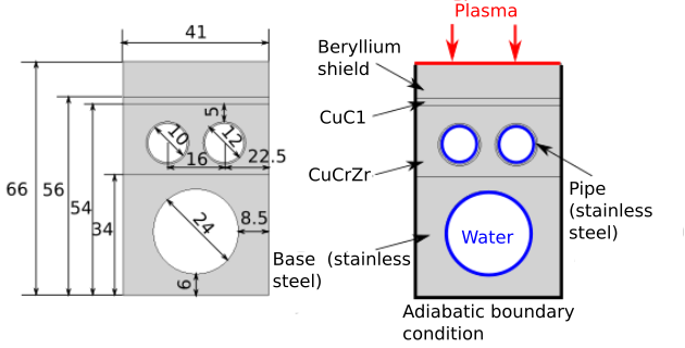
Fig. 3.12 Cross-section of NHF panel with dimensions, components and boundary conditions.

3.2.3.3. Boundary conditions¶

On the figure \(EHF_panelCrossSection\) there is the model of the EHF cross-section with boundary conditions. Beryllium shield is exposed to heat flux comping from plasma. Around the model zero heat flux is defined. Inside the water channel there is bulk temperature \(T_b\) and heat transfer coefficient. Data of heat fluxes on the shield surface are given in SMITER computation that returns power deposition on the panel. Heat transfer coefficient is temperature dependent. Water that is in the channel has bulk temperature of around \(T_b=80\) °C. Graph of heat transfer coefficient with respect to temperature is shown in figure \(EHF_graph_HTC_T\).

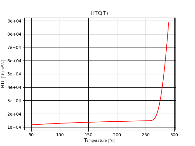
Fig. 3.13 Graph of heat transfer coefficient with respect to temperature.

Heat transfer coefficient is almost constant for temperatures lower than 270 °C. After that it increases rapidly. Heat transfer coefficient of NHF panel is a constant value of \(3000W/m^2K\).

3.2.4. Benchmark study¶

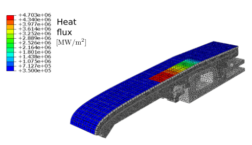
Fig. 3.14 Power deposition on two fingers in EHF panel as defined in the Abaqus study.

Benchmark study for EHF finger was provided by the ITER organisation. Two fingers were studied in this study. Neutron radiation was included into this study as well and was defined as body heat flux. In the Elmer model the body heat source is neglected. Heat flux on surface of the panels has a value of \(350000\text{MW/m}^\text{2}\). One of the finders has additional maximum peak flux has a value of \(4700000\text{MW/m}^\text{2}\). Heat flux distribution is shown in figure Fig. 3.14. Left finger with constant heat flux of \(350000\text{MW/m}^\text{2}\) is known as input finger, because water enters this finger from the tank located in the beam. Right finger is the output finger because the water flows back in the beam tank. With this benchmark study we wsh to compute the temperatures on the surface of simplified EHF panel and compare them to the results of Abaqus study. This way we wish to show that our model is appropriate for more complex plasma distributions. Key question is how to make a simplified model that includes geometry preparation, meshing, boundary conditions and material properties. This model should not be too complex to make and will resemble the real model as much as possible. Very important part of the model is also time computation, that should be as short as possible. Bigger the number of nodes in the study, bigger the computational time. Computational time depends also on the number of steps in the iteration method and error tolerance between two steps. Both of those parameters can be determined in the Elmer FEM program. There is only one cross-section of the simplified finger that does not change along the toroidal direction. For benchmarking purposes the panel can be split into two main cross-sections. For 2D model we define four points on the cross-section, that are shown in figure Fig. 3.15. On those points we compare the temperature with the results of Abaqus study. The differences between the results could be minimized by tweaking the heat transfer coefficient until the temperatures on the simplified model would match the Abaqus results completely.

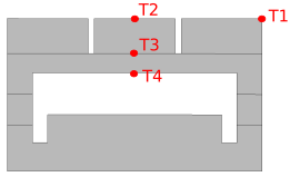
Fig. 3.15 Four points on the cross-section where temperatures were compared.

3.2.4.1. 2D comparison¶

2D model presents only the cross-section of the finger. Boundary conditions and material properties are defined on it. After the calculation we compare the results with the Abaqus study. Two different cross-sections are studied in this benchmark, one with the water tank and the other without the water tank. In EHF panel the water travels through two fingers before it returns to the beam. Temperatures were computed and then compared to the Abaqus results. Results are shown below for each of the four points. The error is given with the equation

(3.32)¶\[\text{abs}\left(1-\frac{T_{elmer}}{T_{abaqus}}\right)*100\]

3.2.4.1.1. Finger out without tank - Results¶

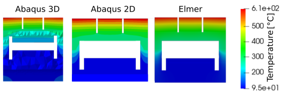
Fig. 3.16 Cross section of finger with water exit to the substructures of the panel without tank.

	Abaqus 3D [°C]	Abaqus 2D [°C]	Elmer 2D [°C]
T1	637.29	607.426	613.53
T2	608.51	592.7	599.46
T3	320	336.4	327.3
T4	255.9	271.39	279.2

3.2.4.1.1.1. Finger out without tank – Error¶

	Error Elmer 2D vs. Abaqus 3D [%]	Error Elmer 2D vs. Abaqus 2D [%]
T1	3.8	1
T2	1.5	1.1
T3	2.1	2.67
T4	8.3	2.9

3.2.4.1.2. Finger in without tank - Results¶

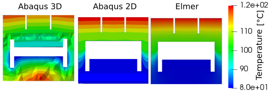
Fig. 3.17 Cross section of finger on the back side.

	Abaqus 3D [°C]	Abaqus 2D [°C]	Elmer 2D [°C]
T1	123.15	124.15	123.97
T2	119.60	123.78	123.61
T3	103.89	109.26	109.14
T4	97.79	105.40	105.32

3.2.4.1.2.1. Finger in without tank – Error¶

	Error Elmer 2D vs. Abaqus 3D [%]	Error Elmer 2D vs. Abaqus 2D [%]
T1	0.7	0.1
T2	3.2	0.1
T3	4.8	0.1
T4	7.1	0.1

3.2.4.1.3. Finger out with tank - Results¶

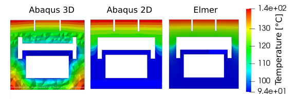
Fig. 3.18 Cross section of finger with water exit at the tank cross section.

	Abaqus 3D [°C]	Abaqus 2D [°C]	Elmer 2D [°C]
T1	137.30	139.00	141.29
T2	133.80	138.61	140.80
T3	117.83	122.30	123.50
T4	112.23	118.56	119.40

3.2.4.1.3.1. Finger out with tank – Error¶

	Error Elmer 2D vs. Abaqus 3D [%]	Error Elmer 2D vs. Abaqus 2D [%]
T1	2.8	1.5
T2	4.9	1.5
T3	4.6	0.9
T4	6.0	0.7

3.2.4.1.4. Finger in with tank - Results¶

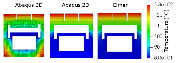
Fig. 3.19 Cross section of finger at the tank position.

	Abaqus 3D [°C]	Abaqus 2D [°C]	Elmer 2D [°C]
T1	123.22	125.44	129.35
T2	119.70	125.12	128.19
T3	101.50	109.20	111.16
T4	97.92	105.40	107.14

3.2.4.1.4.1. Finger in with tank – Error¶

	Error Elmer 2D vs. Abaqus 3D [%]	Error Elmer 2D vs. Abaqus 2D [%]
T1	4.7	3.0
T2	6.6	2.3
T3	8.7	1.6
T4	8.6	1.6

3.2.5. Transformation of panel¶

If we want to map the values of heat flux from SMITER vtk panel onto simplified model of fingers, that is located in the centre of coordinate system, we have to first transform the SMITER panel and position it in a way that it is aligned with the simplified model. In the poloidal direction we have 18 panels. Panels 3,4,5,7,8,9,14,15,16 and 17 are EHF panels and 12,6,10,11,12,13 are 18 NHF panels. Due to the shape of the panels and their position in the tokamak it is much easier to use polar coordinate system. All the panels have the same radial distance r from the origin of the coordinate system. The only change between the panels is height z and angle of rotation \(\varphi\). First the Python code reads the vtk file and stores the data of node coordinates and values of heat fluxes to array. To do that, we need to understand the structure of vtk file.

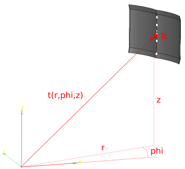
Fig. 3.20 Example of tokamak panel positioned in space with polar coordinates.

3.2.5.1. VTK file structure¶

VTK file format (Visualization Data Toolkit) is a file format that provides a number of source and writer objects to read and write popular data file formats. The Visualization Toolkit also provides some of its own file formats. The main reason for creating VTK data file format is to offer a consistent data representation scheme for a variety of dataset types, and to provide a simple method to com- municate data between software. But if this is not possible, the Visualization Toolkit formats described can be used instead. There are two different styles of file formats available in VTK. The simplest are the legacy, serial formats that are easy to read and write either by hand or programmatically. However, these formats are less flexible than the XML (Extensible Markup Language) based file formats described later in this section. The XML formats support random access, parallel I/O, and portable data com- pression and are preferred to the serial VTK file formats whenever possible. The output of SMITER power deposition calculation is serial text file format, that contains definitions of nodes, triangles and power depositions on nodes in a form of unstructured grid. The format of the files is presented below

# vtk DataFile Version 2.0 [1]
Naslov [2]
ASCII | BINARY [3]
DATASET tip [4]
...
POINT_DATA [5]
n
...
CELL_DATA
n

Head of the file is defined in first line. It contains the version of vtk format. This line is always the same, except the numbers that define the version of vtk format. In the second line one has to define the title of the file. The maximum length of this line is 256 characters. Anything beyond that is ignored by most of the vtk readers. In the third line is the definition of file type, which is either text (ASCII) format or binary format. Then one has to define the datatype of the data sotred in the file. There are six main definitions of datatype in vtk: STRUCTURED_POINTS, STRUCTURED_GRID, UNSTRUCTURED_GRID, POLYDATA, RECTILINEAR_FIELD and FIELD. The datatype of SMITER vtk files is UNSTRUCTURED_GRID. Then one has to write the point data. First line always starts with POINTS, then number of points and then type of data, that is float for SMITER nodes. Unstructured grid means that the file can contain any type of cell. When writing the list of cells, one has to define a special line that starts with CELLS, then number of cells and then the sum of all integers in the cell section. In the following lines we first define the number of identification numbres in the individual cell and then all the identification numbers of the individual elements of cell. One line contains the data for one cell. For example, for triangle we can write 3 id1 id2 id3. The we define a new section where the list of cell types is defined. First line contains key word CELL_TYPES and then the number of all cells. In the next lines we write the type of the element. For example, the identification number of edge is 3, triangle has ID number 5, etc. Then we can write the list of scalar values, that are assigned to each cell. SMITER writes power deposition as scalar value, that is defined on each triangle. This section starts with special line as well. First key word is CELL_DATA and then the number of cells. Second line contains key word SCALARS, then the name of data and then type of data, which is float in SMITER. Last word in this line is the number of all scalar values in an individual cell. In Smiter case just 1. Next lines contain scalar values of heat fluxes. The format is shown below

DATASET UNSTRUCTURED_GRID
POINTS np float
px1 py1 pz1
px2 py2 pz2
...
pxn pyn pzn

CELLS nc 4*nc
3 pID1 pID2 pID3
3 pID4 pID5 pID6
...
3 pIDk pIDm pIDn

CELL_TYPES nc
5
5
...
5

CELL_DATA nc
SCALARS ime float 1
LOOKUP_TABLE default
q1
q2
...
qn

With programming language Python we read the vtk file, that contains heat fluxes. The heat flux is defined in the center of the triangle. We can compute this central point based on the node coordinates \(x,y,z\) of each triangle with ID numbers \(i,j\) and \(k\) in the vtk file.

(3.33)¶\[T_c = \left( \frac{x_i +x_j+x_k}{3},\frac{y_i +y_j+y_k}{3},\frac{z_i +z_j+z_k}{3} \right)\]

Central coordinatees are stored in the Python list of type numpy.array() and are converted to polar coordinates. Now we have to define the mass point of the panel. with the help of functions numpy.amin and numpy.amax we can define minumum and maximum values of \(r,\varphi\) in \(z\) of all coordinates. This way we can get corner values of the panel. Then we can calculate the coordinates of mass point \(T_t\).

(3.34)¶\[T_t = \left( r_{min}+\frac{r_{max}-r_{min}}{2},z_{min}+ \frac{z_{max}-z_{min}}{2},\varphi_{min}+ \frac{\varphi_{max}-\varphi_{min}}{2}\right)\]

Second option for calculation of mass point is to sum up all values of coordinates and then divide with the number of all coordinates. However, in this case the result is dependent on the mesh density.

Now we have to rotate the panel into the origin of the coordinate system in order to overlap it with the simplified model of fingers. First we have to rotate it around z-axis for angle \(\varphi\), so that mass point of the panel lies in the plane xy. Now we can translate the panel in x and y direction so that the mass point is located at the origin of the coordinate system. Last step is to rotate the panel around y-axis. Angle of rotation is hardcoded into Python code and depends oply on the panel position in poloidal direction. The rotation of panels is based on the Euler-Rodrigues formula.

3.2.5.2. Euler-Rodrigues Formula¶

Euler-Rodrigues formula defines the rotation and translation of geometrical objects like vertices, lines, edges, faces, shells and solids. The basic geometric definition is a vertex with three coordinates, usually defined in Cartesian coordinate system. Rotation is defined with four Euler parameters, named after swiss mathematician Leonhard Euler. Rodrigues formula, named after french mathematician Olinde Rodriguesu, is a method of calculating coordinates of rotated points and is used in many other applications like video games and CAD software. Every rotation in space is defined with the angle of rotation and the unit vector, around which the objects are rotated. Euler parameters for rotation are defined as

\(a = \cos{\frac{\varphi}{2}}\)

\(b = k_x\sin{\frac{\varphi}{2}}\)

\(c = k_y\sin{\frac{\varphi}{2}}\)

\(d = k_z\sin{\frac{\varphi}{2}}\)

We notice, that the sine and cosine arguments are two times bigger that the angle of rotation \(\varphi\). If \(\varphi = 360^{\circ}\), the resulting parameters are the opposite values of original parameters \((-a,-b,-c,-d)\). This means that they present the same rotation. If we rotate the geometrical object by angle \(\varphi = 0\), the values of Euler parameters are \((a,b,c,d)=(\pm 1,0,0,0)\). Rotation by \(180^{\circ}\) results in \(a=0\). Sum of squares of all Euler parameters is 1.

\(a^2+b^2+c^2+d^2=1\)

We can rotate the point around an axis with the formula

(3.35)¶\[\begin{split}\vec {x}' = \begin{pmatrix} a^2+b^2-c^2-d^2 & 2(bc-ad) & 2(bd+ac) \\ 2(bc+ad) & a^2-b^2+c^2-d^2 & 2(cd-ab) \\ 2(bd-ac) & 2(cd+ab) & a^2-b^2-c^2+d^2 \\ \end{pmatrix} =\vec {x}\end{split}\]

Euler parameter a has a scalar value, while \(\vec{\omega}=(b,c,d)\) are vector parameters. With standard vector notation the vector formulation of Rodrigues formula is defined as

(3.36)¶\[\vec {x}'=\vec{x}+2a(\vec{\omega} \times \vec{x})+2(\vec{\omega}\times(\vec{\omega}\times \vec{x}))\]

Two rotations around two different axis can be compounded into a composition. Euler parameters of two different rotations are \((a1,b1,c1,d1)\) and \((a2,b2,c2,d2)\). Euler parameters of composition (first rotation 1 and then rotation 2) are

(3.37)¶\[a = a1a2-b1b2-c1c2-d1d2\]

(3.38)¶\[b = a1b2+b1a2-c1d2+d1c2\]

(3.39)¶\[c = a1c2+c1a2-d1b2+b1d2\]

(3.40)¶\[d = a1d2+d1a2-b1c2+c1b2\]

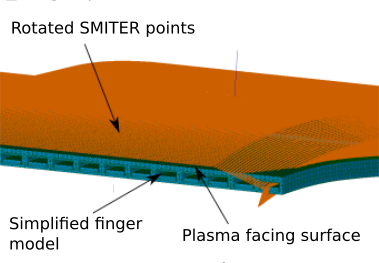
Fig. 3.21 Example of transformation of panel and alignment with the simplified 3D model.

3.2.6. Interpolation of Heat Fluxes¶

When the SMITER surface from vtk file format is aligned with the plasma facing surface of the simplified model, we can map the values of the heat flux from vtk file to the surface of the simplified model. Ideally, the surfaces of vtk file and simplified model should be completely aligned. This is hard to achieve, because different surfaces of panels will be used in the computation of temperature. So it is hard to make a complete alignment of the surfaces.The mapping function is called radial basis function. It is part of the Python library scipy. There are two main approaches on how to map the heat fluxes. We can map the heat fluxes on every finger individually. This means a new mapping function for every finger. It takes a lot of computational time to do that, but the mapping results of heat fluxes match the original ones much metter. The other approach is to calculate just one mapping function for all fingers. This approach is faster but produces less accurate results. Calculation of mapping funciton depends on the size of the interpolation arrays. The size of array depends on the number of nodes that are the basis of the mapping function. If we try to calculate the radial basis function of millions of nodes, our random access memory might not be big enough. In this case we have to use less nodes in out computation. As we see the number of nodes greatly inpacts the calculation of temperatures. The principle used in SMITER is calculation of radial basis function for every individual finger.

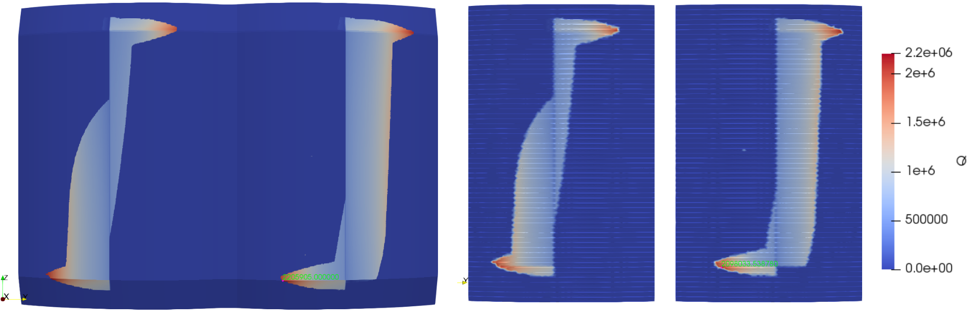
Fig. 3.22 Example of heat flux mapping. On the left side we see the panel of SMITER calculation with power deposition results and on the right side we see the mapped heat fluxes on the simplified model of fingers.

After the calculation of radial basis function we can compute the values of heat flux for every node on the surface of the fingers. Then we have to store those values into sif file, that is the input file for ElmerSolver command. Elmer can read space-dependent boundary conditions. We can write values in the tabular form directly in the sif file, where data is written in columns. However, there are a few limitations when it comes to writing boundary conditions in tabular form. The values of the first column, that is usually the array of x coordinates, must increase, otherwise Elmer fails. Our definition of applying heat fluxes directly on nodes is too complex for such tabular formation of boundary condition. Elmer allows us to define more complex boundary conditions, material properties and solvers with the user defined functions, that can be written and called from sif file. The scripting language of Elmer is Fortran90. This Fortran90 script can be passed as an argument to the appropriate boundary condition section in the sif file. Elmer then calls this user defined function when it needs to. Basis of the script is shown below.

! Definition of function with input parameters Model,
!n and f and output parameter g
FUNCTION myFunction(Model, n, f) RESULT(g)
USE DefUtils
! Definition of properties
TYPE(Model_t) :: Model
INTEGER :: n
REAL(KIND=dp) :: f, g
! Code that computes g
END FUNCTION myFunction

First one can define a function myFunction. Its input parameters are Model, n and f. Property Model is an object of class Model_t and contains node data, boundary condition data and material properties. We can access that data with this object. Parameter f defines time step of the computation and parameter n is the ID number of the individual node that values are being calculated for. When the Elmer program reads the parameters of nodes, it calls this script and defines the ID number of the node as input parameter. Then it executes the script. Example of node access is presented in the code below.

! Definition of properties
REAL(KIND=dp) :: x, y, z
! Reading of coordinates x, y and z
x = Model % Nodes % x(n)
y = Model % Nodes % y(n)
z = Model % Nodes % z(n)

Fortran script calculates all the necessary parameters and returns them in the output argument g. In temperature calculation, the input parameter is the text file, where we stored the heat flux values for every node of the plasma facing surface of simplified finger model. Data of the text file is loaded into script. Then Elmer is searching for the heat flux value of the individual node via the script. Iteration through the list of all values in the file is made. When the ID of the searched node matches the one in the file, the heat flux is stored to variable g and then returned to the Solver. Example is shown in the code below.

! The file is opened. We defined the unit of the file, that can be
! a random integer. We also define the type of access to the data.
open (unit=15, file="fluxdata.dat", status='old',    &
             access='sequential', form='formatted', action='read' )
! Definition of matrix size that will contain data from the file
allocate(list(length_of_list,2))
! Iteration through the file. In every iteration we store the data
! into fortran array.
do i=1,length_of_list
             read (15,*) list(i,1), list(i,2)
enddo
! After we read the data, we can close the file
close(15)
! Then we iterate through the fortran matrix again. If the
! identification number of node matches the input ID, we store the
! flux value into *g*.
do i = 1,length_of_list
             id_vozlisca = list(i,1)
             tok = list(i,2)
if (n == id_vozlisca) THEN
g = tok
end if
enddo

Now we have heat flux defined for every onde on the plasma facing surface of the finger. Other boundary conditions like zero heat flux, heat transfer parameter and bulk temperature is written to the sif file in the tabular form, since these definitions are very simple and not complex like plasma heat flux. These boundary conditions are the same for every finger in the panel. The only change between the panels is the plasma heat flux on the surface. After the computation is done, we get the vtk file for every individual finger as well as one master vtk with all the fingers in it. These files contain temperature distribution.

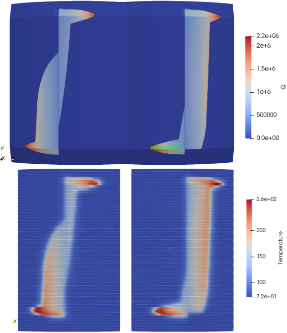
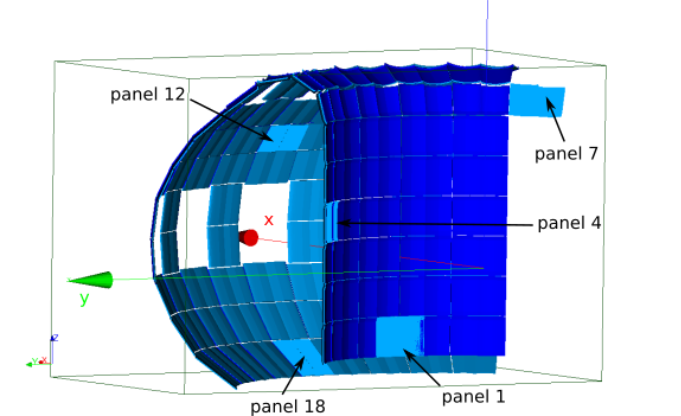
3.2.7. Results¶

The purpose of the Elmer module is to process different types of panels and to calculate the temperature distribution. In this section different ITER panels were tested. Those panels have different locations in space. That is how we tested the translatoin function as well. Panels tested were NHF panels number 1, 18 and 12 and EHF panels number 4 and 7.

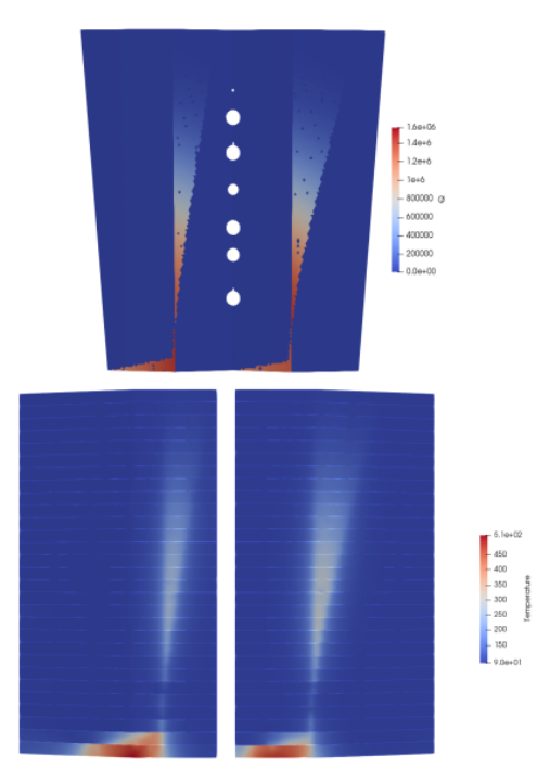
3.2.7.1. Panel 18¶

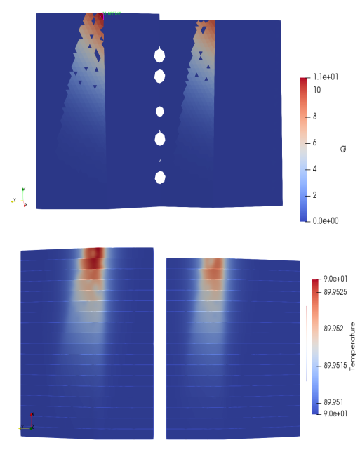
3.2.7.2. Panel 12¶

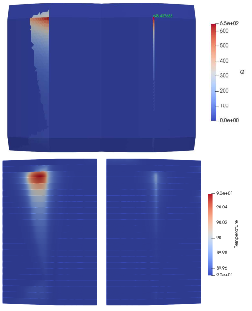
3.2.7.3. Panel 1¶

3.2.7.4. Panel 7¶

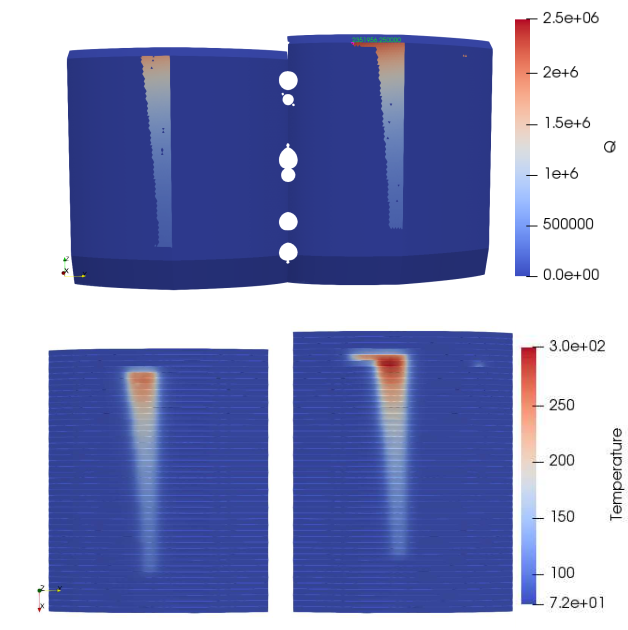
3.2.7.5. Panel 4¶