2.12. Getting LCFS with interpolation
Sometimes an EQDSK G equilibrium contains unhelpful plasma and limiter geometry, that is used for knowing the position of the LCFS. In this case interpolation can be used on the plasma data for finding the LCFS. You can either just plot the LCFS or also export the geometry to SMESH or GEOM.
The method involving interpolation works as follows:
- Load the EQDSK G file
- Read the plasma data, dimensions of the grid and the plasma value at boundary (LCFS)
- Prepare for searching the isocontour by interpolating the plasma data.
- Search for a starting point using bisection
- Calculate the gradient, move perpendicular and add correction.
- Repeat 5 until a full loop is made.
2.12.1. Usage in SMITER
Run SMITER and open the study Test-EQ3-inrshad1-inres1.hdf. Activate
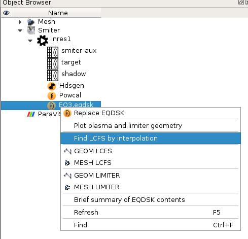
the SMITER module. Right click on the EQDSK object named EQ3.eqdsk
and select Find LCFS by interpolation.
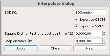
A dialog will open where you can specify whether you wish to export the interpolated LCFS to GEOM or SMESH. Tick them both. There are also two parameters you can edit.
Square Dist. of First and Last point (m^2):
Maximum square distance allowed between the first and last point. This specifies when to stop interpolating the isocontour, i.e., a full loop has been made.
Step distance (m):
Distance of a single step.
Click apply and after a few seconds a plot of the interpolated LCFS will show up and the geometry will also be exported to SMESH and GEOM.