2.13. ITER V3 misalignment¶

In this section, the preparation and computing of some SMITER cases in files nf_55_2023_V3_misalignment.hdf, nf_55_2023_ripple.hdf, nf_55_2023_outer_wall.hdf and divertor_ripple.hdf with SMARDDA are presented. All files with the corresponding magnetic files are available under smiter/study/magtfm, which is our working directory for the following tutorial.

Its special feature is that a 3D vacuum magnetic field is used in addition to the \(\phi\)-independent plasma equilibrium. This allows us to calculate cases with magnetic ripple and also some axially asymmetric misaligned cases. Before running both cases, we need to prepare the 3D \(\phi\)-dependent magnetic vacuum field that is used for field lines when we calculate power deposition on wetted surfaces.

Before you start this tutorial, make sure you have downloaded the two ITER IDMs 47UQUV and Y2KYAD and place them in the current directory. The contents of the two files are explained in the next subsection. Now we unzip both files and prepare the corresponding SMITER cases by:

make

If everything worked, two directories should appear Magnetic field from TFC-Seg01 and MF from TFC CCL misalignments V3_Y2KYAD_v1.0, which correspond to the two zip files.

2.13.1. 3D vacuum field¶

For the calculation of the vacuum field used by SMARDDA for the V3 misalignment, two types of magnetic field files are needed.

The first is the magnetic field generated inside the vacuum vessel by the nominal current flowing in the toroidal field coils. Since this field is generated by 18 coils, it has a 20° periodicity. Therefore, we only need the ripple field in the 20° range for the ‘base file’. In our case, this is the file Magnetic field from TFC-Seg01.dat in the directory with the same name.

The second type are corrections that we want to add to our base file. In principle, these corrections have no periodicity, so we need their values for a full 360°. In our case, they are caused by misalignments of current centrelines “V3” and are stored with the same R-Z grid as the base file, but for the full angle in the files MF from TFC CCL misalignments V3_Y2KYAD_v1.0/Segment*.Dat.

Now that we understand both types of magnetic fields, we will combine themin a .txt file using the Python script full_superposition_field.py. To do this, we need to select the parameters of our input and output files in the script.

First we determine the number of segments (18) and the number of grid points in R, Z and \(\zeta\) directions for both the input and output files.

nr_segments = 18
grid_old = [51, 101, 30]
grid_new = [120, 129, 33]

If different grids are selected, old data will be interpolated to the new grid.

Secondly we choose our input files, name of output file and flags add_fields and for_smardda.

"INPUT:"
base_file = "./Magnetic field from TFC-Seg01/"
base_file += "Magnetic field from TFC-Seg01.dat"
corr_dir = "./MF from TFC CCL misalignments V3_Y2KYAD_v1.0/"
ending = ".Dat"

"OUTPUT:"
output_file = "magtfm360.txt"
add_fields = False
for_smardda = True
#Writes data in reverse order compared to zeta_grid

With the first flag we choose whether or not to add corrections to the base file (in which case we get a ripple field as output). With the second flag we choose whether we want to write the data (and \(\zeta\) grid) in reverse order in toroidal direction.

Note

SMARDDA uses the grid \(\zeta\), which is defined clockwise from top to bottom, so that the data is in reverse \(\phi\) order.

Sript uses numpy and scipy, these modules must be loaded before running Python script. After you have edited the script and loaded modules, simply run it by:

python full_superposition_field.py

Now we have a 3D field file *.txt, which is used to calculate the following cases.

Alternatively you can also run this script in SMITER under Tools‣Plugins‣3D-Vacuum Field with the same parameters as before. The output vacuum field file will appear in the study/magtfm subdirectory.

To use the new magnetic file, you must right-click on the previous magnetic file in SMITER case and select Change MAG file.

2.13.2. Ripple¶

This subsection presents the calculations and results of the file nf_55_2023_ripple.hdf. It focuses on the calculation and comparison of the power load on the single (FW4) panel with (case ripple) and without the ripple field (no_ripple). The ripple magnetic field was calculated using the Python script from the previous subsection with the flags add_fields=False and for_smardda=True.

As the name of the file suggests, it comes from case nf_55. This means that most of the CTL parameters are the same for both included cases. However, we are not interested in observing the target at an R different than the shadow. Therefore, we also need to shift it by -5 mm in the X direction before rotating it to create a 360° target.

The main difference between the two cases described is that the ripple case has an additional mag file describing the 3D ripple field. For our mag file we choose the following parameters:

data_layout: 12

for ITER specified data (magnetic field),

i_requested: 32.68

\(B_{T}R\) to determine nominal value (5.3T) of toroidal magnetic field at R specified at

radius_of_axis: 6.16.

If an error occurs in the Powcal due to inconsistent currents, this value should be corrected (it must match values in the Equillibrium file).

Now we must specify starting angle of out magnetic field in [°] with

zeta_start: -9.9.

In addition, we must use the following for cases with an additional vacuum field use

beq_fldspec: 3

in the shadow and target CLT parameters.

At the end make sure to use

calculation_type: ‘global’

for cases where you need more than full angle fieldlines.

Now both cases can be run and compared. In Fig. 2.35 we see the result of the calculated power loads for the ripple magnetic field.

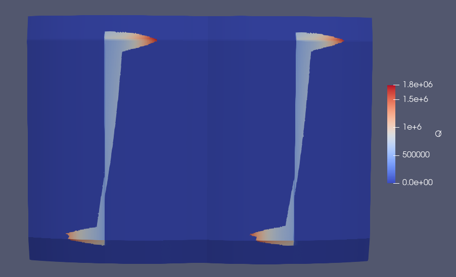
Fig. 2.35 Calculated power loads for the ripple magnetic field.

In Fig. 2.36 we compare both results by subtracting the heat fluxes of the two cases. The subtraction was carried out in Paraview in SMITER. A detailed description of the procedure can be found in the next subsection.

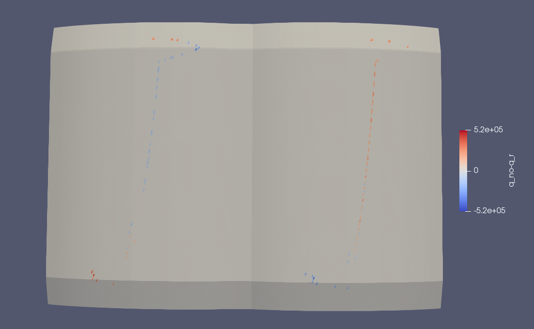
Fig. 2.36 Difference of the calculated heat flux with ripple field compared to field without ripple.

As we can see, there are minimal differences between the two cases. Since the ripple field is not significantly different compared to the axisymmetric ideal field, such differences are to be expected. Now we are interested in simulating cases with a more disturbed magnetic field. An ideal example is the case of V3 misalignment.

2.13.2.1. Diference between two cases in Paraview¶

To see the difference between the heat loads for different cases on the same grid, we need to use some Paraview filtres. First we need to rename the quantities we want to compare in both cases. This is necessary because we cannot compare two quantities with the same name. The described renaming can be done with the Calculator filter. Then we use ctrl + shift to select both cases and use the filter AppendAttributes to merge all the quantities into a single dataset. At the end we have to apply the filter Calculator again to subtract the two (previously renamed) heat loads.

In Fig. 2.37 we see how using of described filters in Paraview should look like at the end.

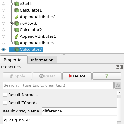
Fig. 2.37 The Paraview filter tree used for comparing two cases.

2.13.3. V3 misalignment¶

Finally, we have arrived at the main file of our interest nf_55_2023_V3_misalignment.hdf. It contains four cases: v3_misalignment for FW3, FW4, FW5 and no_misalignment for FW4. The 3D magnetic field for the case without misalignment is the same as in the case ripple, again the second magnetic file was calculated with the Python script from the previous subsection with the flags ‘add_fields=True’ and ‘for_smardda=True’.

Now we have to select the CLT parameters, which must be the same as in the ripple field case described earlier. Then we can run all the cases and examine the results.

In Fig. 2.38 we see the results of all three misaligned cases (FW3-5), with the wetted areas similar to those of the previous cases.

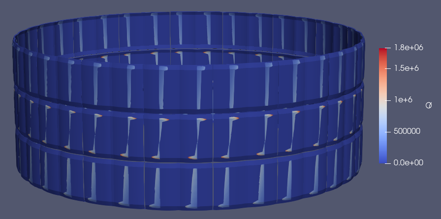
Fig. 2.38 Heat loads on FW3-5 for V3 misaligned magnetic field.

At first glance, the results on FW4 look exactly like the results in the no_misalignment case. To see the difference, we again perform the subtraction of both heat loads in Paraview. The result for FW4 is shown in the figure Fig. 2.39.

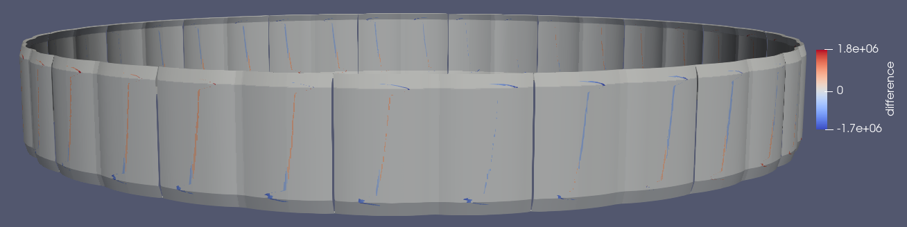
Fig. 2.39 The difference in heat loads between cases with and without V3 misalignment.

As we can see, a misaligned V3 magnetic field actually produces somewhat different results than a pure ripple field. In general, it looks like the magnetic field contracts a little in one direction and extracts in the other, resulting in a slightly larger or smaller wetted area on FW4. This behaviour looks approximately periodic, with a 180° periodicity which is consistent with the final report on the distortion of the plasma boundary due to the misalignment of the centreline of the TF coils, which is associated with our IDM data for the mangetic field.

2.13.4. Ripple on outer wall and divertor¶

The further we are from the central axis of the tokamak, the greater the change in the magnetic field caused by the ripple. It is therefore useful to also observe the effects of the ripple on the heat fluxes on the outer wall. This was done for FW 12-17 in nf_55_2023_outer_wall.hdf.

Again, the case comes from case nf_55 and therefore shares the equilibrium file and all CTL parameters with the previous case, but has a different target and shadow geometry. The results for outer wall geometry with and without ripple can be seen in the figure Fig. 2.40.

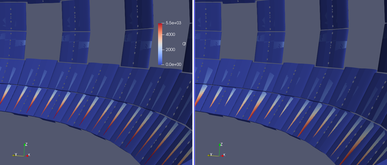
Fig. 2.40 Heat loads on outer wall cases without (left) and with (right) ripple.

The first thing we can notice is that the heatloads are much smaller compared to the heatloads on the inner wall. This is because the LCFS for our equilibrium touches the inner wall, but not the outer wall, which is a few decimetres away. As we can see, the effect of the ripple on the outer wall can be seen even without using different paraview filters and subtracting the results. The wetted surface changes with a periodicity of 20°, as expected, but the maximum values of the heat flows do not change significantly.

To make the effect of the ripple field even clearer, it is useful to compare the angles of impact of the fieldlines on a small scale rather than (heatload) on a full scale. This is because where the wetted area changes a little, the maximum value of these areas is much greater than the direct ripple effect (change in angle). The observation of the impact angles was done with divertor_ripple.hdf for the divertor geometry because the effect is best seen here.

Again, we calculate the ripple case using the ripple field magnetic file. Before the calculation, we need to make sure that the vacuum field makes sense for our equillibrium file. In our case, this was artefficially done by setting

i_requested: -35.52

Now we can calculate both cases and compare the angles of incidence as explained earlier for the difference in heatload in the paraview. To see the ripple effect better, you can use Hoover Cells On at a certain height and different \(\phi\) to find a reasonable range, and then use Rescale to custom range on the data. The colouring of the surface depending on \(\phi\) should appear with about 0.1° difference between minimum and maximum. The results can be seen in the figure Fig. 2.41.

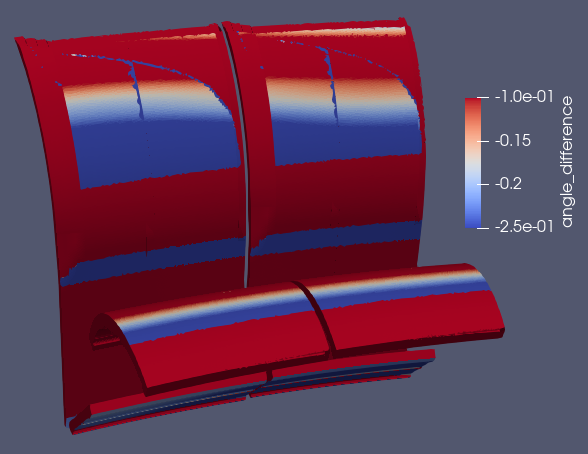
Fig. 2.41 Angle difference on divertor between cases with and without ripple.

To further examine the ripple effect we can make another graph from the data we have obtained. This time we will plot the angle difference as a function of \(\phi\) at the chosen altitude. Again we prepare our data using the paraview filter. This time we use the Slice filter for the previously calculated angle difference. In the filter properties we have to make sure that the data is sliced horizontally, i.e. the normal in Z-direction has to be used. For better results, we can use cylindrical Clip to obtain data on the mostly wetted inner surface only.. Then we use CellDataToPointData filter and Save data as *.csv file in working directory and make sure that we only select both angles (angle with ripple, angle without ripple) in the array selection.

Now we can use another Python script plot_difference.py to plot the results. It plots the difference for the most recent *.csv file in the directory. You can see the results in the figure Fig. 2.42.

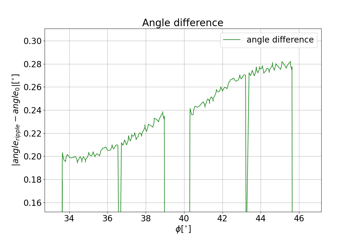
Fig. 2.42 Graph of the angular difference between cases with and without ripple as a function of \(\phi\).

As we can see, a sin-like line appears with some zero values. These zero values occur at \(\phi\) where the surface is not wetted and therefore no real fieldlines appear here and so there is no angle of impact.

Now we can calculate the divertor mesh with a finer meshing. In these cases the calculation times are very long (several hours), so it is advisable to use MPI if possible. The results of such a calculation can be seen in the figure Fig. 2.43.

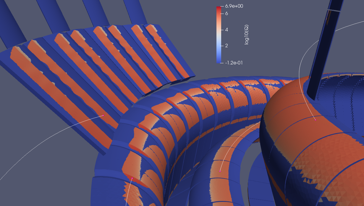
Fig. 2.43 Wetted surface on divertor for 3D ripple field. The effect of the ripple can only be seen at the very top of the divertor, where the edge of the wetted area oscillates for a few centimetres along the \(\phi\).