4.16. SMITER-PFCFLUX benchmark ‘Faraday screen bars’
4.16.1. Introduction
The purpose of the “Faraday screen bars” case is to benchmark SMITER software withan existing field line tracing software PFCFLUX, developed at CEA, Cadarache and to give re-evaluation of the incident heat load on the Faraday screen. Case was first re-run with PFCFLUX solver with set-up,prescribed above. Then the full case was repeated with SMITER GUI. The goal was to obtain similar results with respect to PFCFLUX. The PFCFLUX case description is available in ITER IDM document “Evaluation of the incident heat flux on the Iter ICRH Faraday screen” with ID B5AYHG. The document contains multiple Faraday screen bar cases. The case relevant for this benchmark is a case with limiter plasma 7.5MA SU OUTBORD.
Faraday screen is composed of 4 frame quadrants, as shown in Fig. 4.46. Each one of them is an assembly of 16bars. The bars are the components facing the plasma. The bars have their front face shaped as a gable roof. At a nominal position the Faraday screen bars are recessed outward the plasma by \(10mm\) from the FW poloidal profile. This position guarantees a protection from plasma by the neighbouring FW panels. However, the neighbouring first wall panels do not provide full shadowing of the bars and some area of the bars remains exposed.
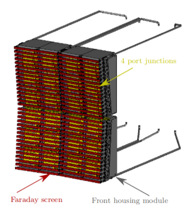
Fig. 4.46 Front side of ICRH screening with Faraday screen.
4.16.2. Input data
4.16.2.1. Equilibrium
The equilibrium used is EQDSK-G Limiter_7.5MA_outbord.EQDSK with the following specifications:
- Plasma current: \(I= 7.5MA\)
- Nominal toroidal magnetic field: \(B_T = 2.65T\) at \(R= 6.2m\).
- Magnetic pitch: \(B_{\theta}/B_{\Phi}= 0.154\)
The contour plot of magnetic flux (\(\psi\)) values with LCFS and LIMITER wall for the equilibrium file used is shown in Fig. 4.47.
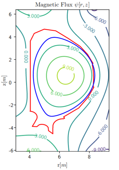
Fig. 4.47 The contour plot of magnetic flux (\(\psi\)) values with LCFS and LIMITER wall.
4.16.2.2. Meshes
The target are the Faraday screen bars. Front surfaces of Faraday screen, that can be reached by the plasma, are shown in Fig. 4.48:
- Beryllium (Be) front face
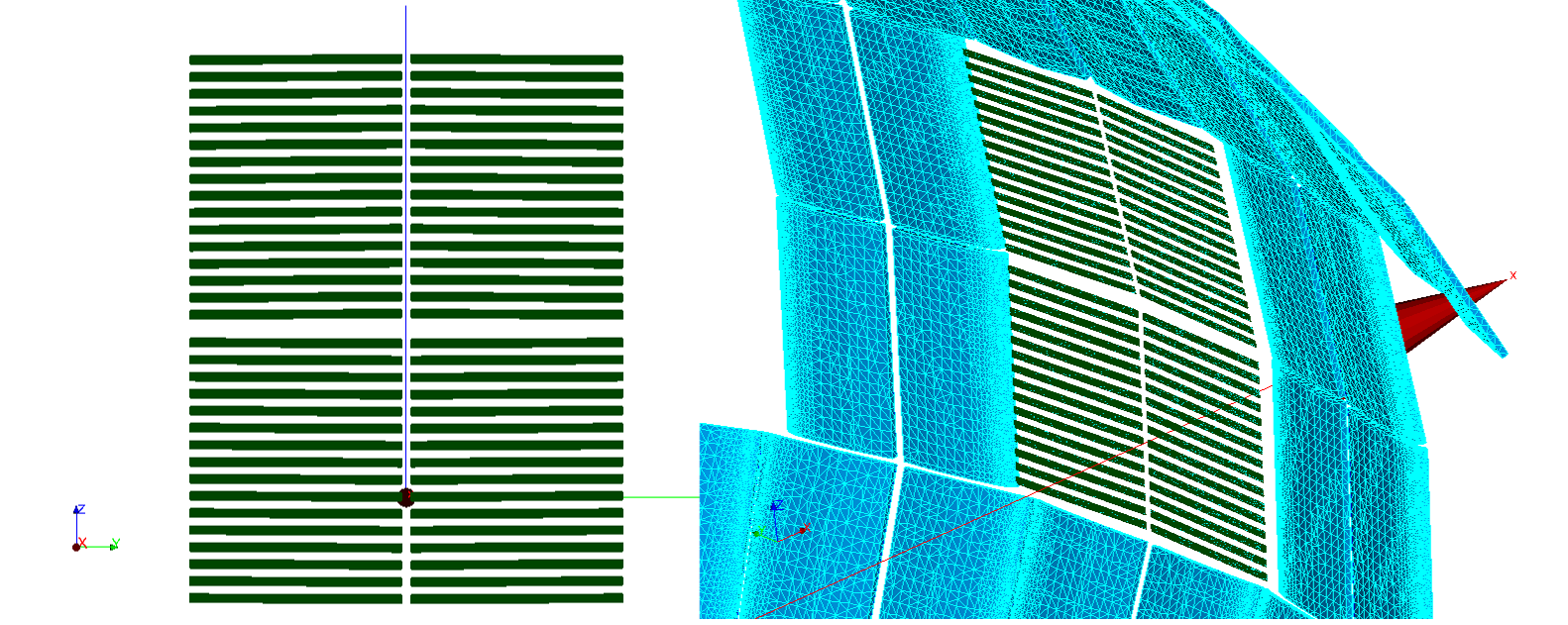
Fig. 4.48 Target mesh.
Shadow mesh is comprised of neighbouring panels that shadow the Faraday screen bars. In current case the shadow mesh is shown in Fig. 4.49:
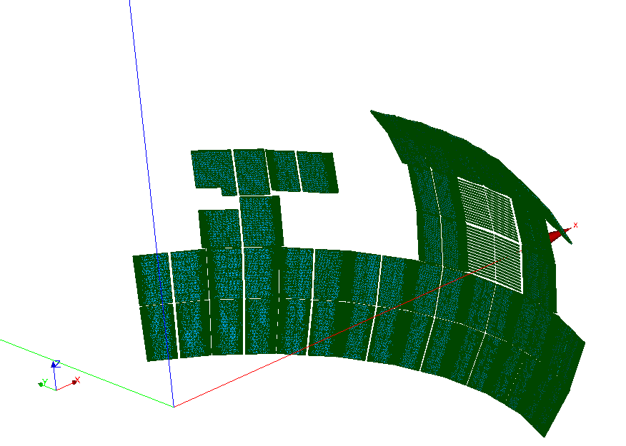
Fig. 4.49 Shadow mesh.
The bars are meshed with triangular elements. Size of each triangle on the target mesh is \(2mm^2\). Triangles of surrounding shadowing panels vary from \(2mm^2\) to \(1244.1mm^2\). There is no misalignment between panels, so the nominal position is considered.
4.16.3. Setting up the SMITER case
The study ITER_IDM_B5AYHG_benchmark already contains target and
shadow meshes and no additional action needs to be taken here. The meshes are
- surf_be: front layers of Faraday screen
- Bm_mesh_surf_be: Surrounding meshes, including the surf_be target mesh.
- LIMITER-Limiter_7.5MA_outbord.EQDSK: Limiter wall contour
In SMITER two starting parameters are neccessary in order to run the computation. One is the power decay length at midplane (m), \(\lambda_m>0\) and the oter is either power loss \(P_{loss}\) of parallel heat flux at outer midplane \(q_{0}\).In case of the presented benchmark study these parameters are as follows: * Decay length: \(\lambda_m = 24mm\) * Heat flux at outer midplane: \(q_0= 29MW/m\)
4.16.3.1. GEOQ parameters
In the SALOME Object browser in SMITER section under “7_5_MA_SU_OUTBORD” case, one can right click on either target object (surf_be) or shadow object (Bm_mesh_surf_be) and select Edit CTL.
Under beqparameters one can observe following parameters
| Parameter | Value | Description |
|---|---|---|
| beq_bdryopt | 15 | \(\psi_m=\psi_{ltr}\) Boundary based on nodes of geometry, outboard values are used for \(R_m,B_{pm}\) and \(B_m\) |
| beq_cenopt | 4 | Read the center values of R and Z from eqdsk file |
| beq_fldspec | 1 | Use flux coordinates |
| beq_nzetap | 1 | Fieldlines might go around torus! |
Note
The beq_bdryopt option used in this case is 15, which implies
calculation of reference magnetic flux value \(\psi\) that is
based on nodes of given target and shadow mesh. In this case, the
beq_psiref parameter is ignored.
4.16.3.2. HDSGEN parameters
Refer to general setting parameters for limiter cases for HDSGEN .
4.16.3.3. POWCAL parameters
| Parameter | Value | Description |
|---|---|---|
| calculation_type | local | ‘local’ shadowing only by toroidally localised geometry |
| shadow_control | 1 | Enable shadowing |
| q_parallel0 | 29000000 | Parallel heat flux at outer midplane (in \(W/m^2\)) |
| power_split | 1 | power split ion to electron direction. |
| decay_length | 0.024 | decay length in meters. |
Note
The power_split parameter should be specified to 0.5 when
power_loss is activated. In case of q_parallel0, this
parameter should be specified to 1. To enable either q_parallel
or power_loss, the enabled parameter should have a positive
value and the disabled parameter should have a negative
value. Check the power_loss parameter in the current study (set
to \(-7.5MW\)).
4.16.3.4. Run case
To run the case, right click on object 7_5_MA_SU_OUTBORD and
select Compute case.
4.16.4. Results
In the following study, power deposition is studied only on the front surface, without poloidal and toroidal layers. The front peak heat flux, calculated with PFCFLUX, is \(0.766MW/m^2\). It is shadowed when taking into account the neighbouring blanket modules. The front peak is then \(0.703MW/m^2\). Similar results are obtained with SMITER field line tracer. The peak of the front surface is \(0.701MW/m^2\). Results are shown in Fig. 4.50.
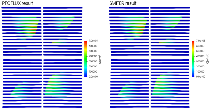
Fig. 4.50 Power deposition in PFCFLUX (left) and SMITER (right). Blue area represents 0 power deposition on the Faraday screen bars. Wetted area in SMITER matches the PFCFLUX well.
Next step is to compare actual differences between power deposition values. The same target grid was used in both solvers. PFCFLUX returns power deposition values on nodes of the mesh, while SMITER calculates power deposition on the cells, in this case triangles. Assuming that the power deposition is defined in the center of the triangle, one can average power deposition values of PFCFLUX to the center of the cell by taking into an account the power deposition values on all three nodes of the triangle and average them. The formula for calculation of percentage error is then
\(err=100*|1-\frac{q_{smiter}}{q_{pfcflux}}|\)
Visualization of errors is shown in Fig. 4.51. Average power deposition error between values is around 1%. Same percentual error was calculated for magnetic flux values. The average difference for magnetic flux is around 0.1%.
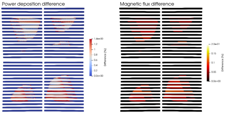
Fig. 4.51 Left: Percentual difference in power deposition for both field line tracers. The average difference is around 1%. Right: Difference in magnetic flux \(\psi\). The average difference between magnetic flux values calculated in both fiedline tracers is around 0.1%.