4.20. Power deposition on ICRH antenna for ELM and SS profile
4.20.1. Power deposition model
4.20.1.1. Edge localized mode profile
The power deposition mapping onto FWPs 8-18 and ICRH Faraday screen can be described with two main contributors, edge localized mode (ELM) and the steady state, inter-ELM profile. Development of ELM power deposition profile is based on development of average density and temperature of an ELM filament using 0-D fluid equations [2]. Following the power balance one obtains
Equation 2 corresponds to maximum ELM-averaged parallel heat flux density evaluated at the OMP. Expression \(w_{fil}/w_{fil0}\) is the fraction of the ELM energy that reaches a given radial distance from the first separatrix, w_fil is the poloidal filament width, w_fil0 is the energy loss per ELM, \(f_{ELM}\) is the ELM frequency, \(R_{OMP}\) is the radius at the OMP, \(\lambda_{q_{||}}\) is the local ELM energy decay length, \(n_{fil}\) is the number of filaments per ELM, \(B_p\) is poloidal component of B-field at OMP, \(B_{tot}\) is the magnitude of B-field at OMP. The expression \((B_p/B_{tot})_{OMP}\) represents magnetic field line pitch angle at the OMP, and \(d\) is the poloidal separation of the filaments, where one assumes \(w_{fil}=d/2\). The factor \(1/1.7\) accounts for strike of filaments on the first wall at random toroidal position. Constant parameters for ELMs are \(w_{fil0}=1MJ\), \(f_{ELM}=40Hz\), \(n_{fil}=10\) and \(d=0.6m\). To solve the equation 2 one must obtain the missing parameters \(w_{fil}/w_{fil0}\) and \(\lambda_{q_{||}}\). Their computation is based on development of average density and temperature of an ELM-filament using 0-D fluid equations of the parallel filament transport [4]. The filament transport is described in the filament frame of reference by evolution of a Gaussian structure in which the initial particle and energy content decreases due to parallel losses along the flux tube connecting two solid surfaces. Energy sink rate is proportional to \(c_s/L_{||}\), where \(c_s\) is the ELM filament ion sound speed and \(L_{||}\) is the connection length given as a function of distance from the first separatrix. Connection between radial distance from the beginning of the filament, which starts at \(R_{OMP}\), and filament evolution time is given through the velocity of the radial filament propagation, \(v_r\). This model has been found to have a good agreement with experimental observations [4]. In this paper it is assumed that the ELM filaments are ejected into the SOL from the 1st separatrix with temperatures and densities equal to half of the pedestal top values \((T_{i,ped}=T_{e,ped}=5keV\), \(n_{e,ped}=7.5e^{19} m^{-3}\). The velocity of ELM for the model is given as \(v_r=500m/s\). Equation 2 assumes that all filaments are launched into the SOL at the OMP and thus neglect the poloidal spreading of the filaments. The connection lengths \(L_{||}\) at the OMP are calculated using the SMITER field line tracer. Components of magnetic field \({B_p}\),:math:{B_tot}, needed for evaluation of the equation 2 are calculated by SMITER. SMITER evaluates magnetic field components at OMP based on the input poloidal magnetic flux. Once the power deposition profile is calculated with the ELM model, one can calculate the power deposition on the target. The calculation is given as
where \(\Delta r\) is the distance between the triangle barycentre and the first separatrix at outer midplane, \(R_{sep1OMP}\) radius of the first separatrix, \(R_b\) is the barycenter of the triangle and \(\alpha\) is the impact angle of the field line hitting the triangle.
4.20.2. Steady state profile
The plasma profile used in the inter-ELM (\(\lambda=0.17m\)) and ELM (\(lambda=0.005m\)).
Parameters:
- Near SOL decay length: \(\lambda_n = 0.005 m\)
- Far SOL decay length:\(\lambda_f = 0.17 m\)
- Breakpoint SOL: \(R_b = 0.025 m\)
- Power loss: \(P_{sol} = 100 MW\)
Power deposition profile for \(\Delta r < R_b\):
Power deposition profile for \(\Delta r > R_b\):
Results for 4, 6, 8 cm shift:
Equilibrium file: geqPullTo8cmDsep8cm_00000_RDHR.eqdsk ICRH-optimized plasma equilibria are shifted outwards with respect to the Baseline equilibrium for 10 cm.
4.20.3. Heat load calculation
Heat loads are calculated using the field line tracing software SMITER. Connection lengths were first obtained through this code, since they are an input parameter to the ELM loss model that calculates the power deposition profile. Connection lengths are calculated starting from the outer midplane towards the outward panels. Full 3-D geometry is taken into an account and serves as a shadow for the field line tracing calculation. If the field line hits the shadowing triangles, it is terminated and its length from the starting point to the end is calculated. Connection length profile changes as the equilibrium is shifted towards the outer targets. Connection lengths can be calculated in two directions, towards the outer or the inner targets. In this paper, the shortest of the two was taken as the input to the ELM loss model, since it represents the strongest sink of the parallel energy to the target. The connection length plot is shown in Fig. 2.
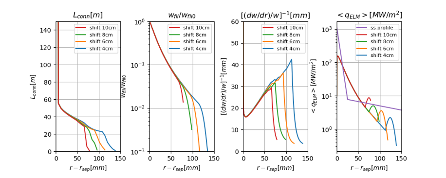
Fig. 4.70 Compilation of results of ELM model for the ICRH-optimized configuration with \(\Delta OMP=4,6,8\) and \(10cm\). From left to right: Connection lengths, ELM filament energy normalized to the inital energy, filament energy decay length, and the maximum ELM-averaged heat flux with the steady state profile. All parameters are plotted against the distance from the 1st separatrix at the OMP.
Moreover, different ELM filament velocities and frequencies were tested to give a framework within the FWP and ICRH screen limits would not be exceeded. The range of ELM velocities is given between \(250m/s\) and \(1000m/s\) and the frequencies are given between \(30Hz\) and \(60Hz\). Different configurations were then performed for different velocities and frequencies. The plot of ELM profile for different filament velocities and frequencies is shown in Fig. 4. One can notice that for the short distances from the OMP, the heat flux profile is increasing rapidly with both frequency and velocity of the filament, however, in case of the velocities the drop for slower filaments is not as fast as for the faster ones. From these different configurations, power depositions on ICRH Faraday screen and FWPs 8-18 were calculated and the increase in peak power depositions as a function of frequencies and velocities can be seen in Fig. 4.
4.20.4. Radiation
The purpose of this section is to calculate power load on the ICRH Faraday screen and first wall panels 8 - 18 following the electron emission of the plasma. Radiation profile is given as a 2-D distribution in R-Z direction and is assumed to be constant in toroidal direction. The profiles were calculated with JINTRAC code [8] that solves the electron energy transport equation. The radiation profile is given in Fig. 5. Calculation of heat fluxes is based on ray-tracing algorithm, where the finite number of rays is projected into space from every triangle of the ICRH mesh. The path of every ray is then traced and if the ray does not hit any light source (plasma), the contribution of this source to the total power on the triangle is 0. If the ray goes through the plasma, the contribution of power to the total power is calculated through Monte-Carlo integration of plasma source on the part of the path that is in the plasma source. One third of tokamak was used in the study. Since the plasma source is constant in toroidal direction, mirror is implemented on both sides of the tokamak, so that rays are reflected back with the full specular reflection. Due to the axisymmetry, only upper right quarter of the Faraday screen is used as the observer for the radiation calculation, as well as the straps behind it. The surface of the panels and divertor is fully absorbing. This means that the ray is terminated, if it intersects the triangles of panel and divertor mesh. The radiation source is poloidally homogeneous. This may not be the case in particular for radiation
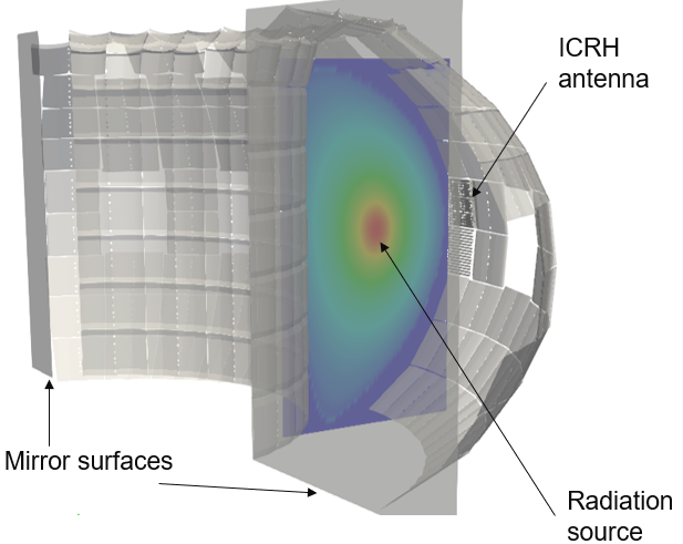
Fig. 4.71 Case setup of the ray tracing studies.
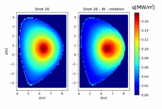
Fig. 4.72 Plasma source is constant in toroidal direction. First case is axisymmetric around the plasma core. In the second case, a factor due to W-rotation is added to the source and the radiative power of the plasma increases.
due to tungsten rotation. As an approximation of this effect the W-rotation factor \(\exp{M^* (\rho,\theta)/2}/<\exp{M^* (\rho,\theta)/2}>\) is applied to the given power density [9]. Here, \(M^*\) is the Mach number, given by \(M^* (\rho,\theta)=m^* \Omega(\rho)^2 R(\rho,\theta)/T_i(\rho)\), where \(m^*\) is the effective impurity mass, \(\Omega\) is the angular frequency of toroidal plasma rotation, \(R(\rho,\theta)\) is the major radius and \(T_i (\rho)\) is the ion temperature.
4.20.5. Results
Peak power depositions for ICRH antenna for different shifts with the configuration of \(f_{ELM}=30Hz\) and \(v_{ELM}=500m/s\) is shown in Table 1. One can notice that for the steady state profile the increase in power deposition is almost linear, while for the ELM profile the power deposition starts increasing fast after reaching \(6 cm\) of shift. For smaller shifts, the impact of the steady state profile is higher as one can see from rightmost plot of Fig. 3, where the steady state profile from the SOL breakpoint is decreasing slowly. As the equilibria is moved forward, the impact of ELM profile gets bigger. Wetted area and power deposition plot on ICRH antenna for different shifts is shown in Fig. 7. Wetted area is increasing as the equilibria is shifted towards the antenna. The peak power deposition appears on lateral tiles due to higher impact angle of the field lines, while the vertical tiles receive smaller thermal loading. The angle of the field lines striking the lateral surfaces of the bars is around \(20°\), while for the front surfaces the angles are around \(3°\). One can notice that the high power deposition can be observed on panels 8, 9, 14, 15 and 18. Of those 5 panels, the peak power depositions are on panels 8 and 15. Power deposition for different shifts for ELM and steady state profile are seen in Table 1 for ICRH antenna and in Table 2 for panels 8 and 15. Peak radiative heat load of \(0.045 MW/m^2\) on the FWPs can be observed on panel 15. Panel 15 is also the closest panel to the core of the plasma as seen in Fig. 5. The lowest power load of \(0.000086 MW/m^2\) is received by panel 8, which is also the panel with the furthest distance from the radiation plasma core. Peak power load of \(0.041 MW/m^2\) on the ICRH Faraday screen is on the front bars for the axisymmetric radiation profile. The straps behind the Faraday screen receive a maximum power load of \(0.023 MW/m^2\). When the rotation of tungsten is taken into an account, the peak power deposition on panel 15 is \(0.13 MW/m^2\) and on ICRH Faraday screen bars is \(0.12 MW/m^2\). Peak power load on straps in case of W-rotation factor inclusion is \(0.065 MW/m^2\).
| Peak values on ICRH antenna Faraday screen |
|
|
|
|
|
|
|---|---|---|---|---|---|---|
| Shift 4 cm | 0.68 | 0.7 | 0.12 | 0.168 | 1.38 | 0.29 |
| Shift 6 cm | 1.09 | 0.79 | 0.18 | 0.2 | 1.88 | 0.38 |
| Shift 8 cm | 1.5 | 0.88 | 0.28 | 0.23 | 2.34 | 0.51 |
| Shift 10 cm | 2.67 | 1.0 | 0.87 | 0.26 | 3.67 | 1.13 |
Table 2: Maximum power deposition values on ICRH antenna.
| Peak values on FWPs 8 - 18 |
|
|
|
|
|
|---|---|---|---|---|---|
| Shift 4 cm | 2.43 | 1.5 | 0.48 | 1.45 | 0.25 |
| Shift 6 cm | 2.47 | 1.59 | 0.6 | 1.9 | 0.38 |
| Shift 8 cm | 3.5 | 1.72 | 0.9 | 3.36 | 0.9 |
| Shift 10 cm | 4.80 | 3.2 | 2.2 | 8.8 | 1.5 |
Table 2: Maximum power deposition values on panels 8, 9, 14, 15 and 18 for both ELM configuration of \({f_{ELM}=30Hz}\) and \({v_{ELM}=500m/s}\) and steady-state profile.
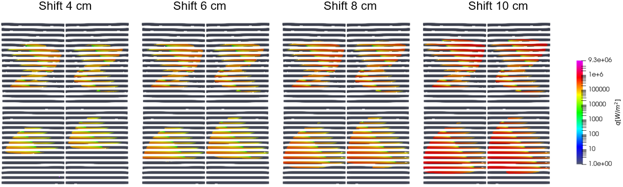
Fig. 4.73 Power deposition on front bars of ICRH Faraday screen for (a) 4 cm shift, (b) 6 cm shift, (c) 8 cm shift and (d) 10 cm shift. The wetted area on the screen is increasing as the plasma equilibria is shifted towards the antenna. The peak power deposition appears on the bar 10 in the upper left quadrant of the Faraday screen. In the bottom figures the power deposition on the lateral bars can be seen for (e) 4 cm shift, (f) 6 cm shift, (g) 8 cm shift and (h) 10 cm shift. Peak power depositions are given in Table 1.
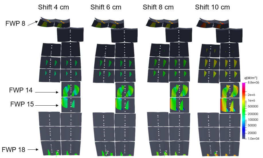
Fig. 4.74 Power deposition and wetted area on FWPs 8-18. FWPs 8 and 15 receive most power loading as seen from the plots.
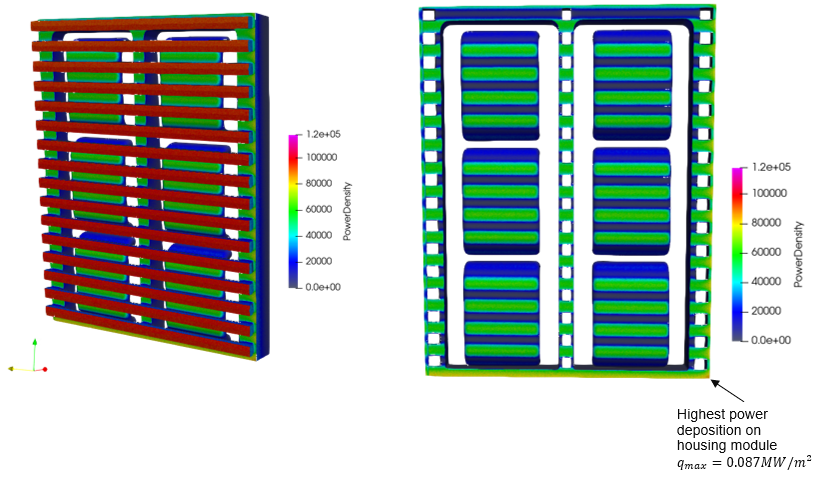
Fig. 4.75 figure 6: (a) Radiative heat load on the FWPs 8-18. Maximum power load of \(0.045 MW/m^2\) can be observed on panel 14. Panel 14 is also the closest panel to the core of the plasma as seen in Fig. 5. The lowest power load of \(0.000086 MW/m^2\) is received by panel 8. (b) Power load on the ICRH Faraday screen. Maximum power load on front bars is \(0.041 MW/m^2\). (c) The straps behind the Faraday screen receive a maximum power load of \(0.023 MW/m^2\). (d) Radiative heat load on the FWPs with inclusion of W-rotation factor. Maximum power deposition on panel 14 is \(MW/m^2\). (e) Maximum power deposition on ICRH Faraday screen bars is \(0.12 MW/m^2\). (f) Maximum power load on straps in case of W-rotation factor inclusion is \(0.065 MW/m^2\).
Power flux densities on FWPs 8-18 and ICRH Faraday screen have been presented. ICRH Faraday screen is well protected by the neighbouring panels in the baseline scenario. In this paper, the equilibria was shifted towards the plasma by 4,6,8 and 10cm. To account for the realistic 3-D geometry of the ITER tokamak, where the PFCs are shaped in the way to avoid exposed edges in the case of misalignment, sophisticated magnetic field line tracing environment is used to determine the factors for accurate calculation of factors that influence the calculation of power deposition on ICRH screen and outboard panels. Once the field line tracing is determined, two different power deposition profiles, ELM and steady state model are combined to calculate the power deposition on the ICRH Faraday screen and outboard panels 8-18. Power deposition for the ICRH antenna is beyond the limit of \(3 MW/m^2\) for the shift of up to 8 cm. Higher shifts lead to fast increase of power deposition on the lateral faces of the Faraday screen. According to the field line tracing results in this report, the field lines do not penetrate behind the beryllium structures of the Faraday screen. Bigger concern present the results on the FWPs. Panel 8 receives a power deposition up to \(3.5 MW/m^2\) in the 8cm shift and needs careful monitoring by the tokamak operators. In case of baseline equilbrium, no field lines strike the panels 14 and 15. As the plasma is shifted towards the outer targets, power deposition increases especially on the edges of the panel 15 due to high striking angle. At 8 cm shift, the peak power deposition increases to \(3.6 MW/m^2\). At 10 cm shift, the power deposition is over \(8 MW/m^2\). The impact of the radiative heat fluxes on the ITER Faraday screen and FWPs 8-18 is also presented in this paper. The peak values of the radiative heat fluxes are much lower than the fluxes doming from the thermal power of the plasma. However, they need to be properly assessed as well. The approach used in the paper is to calculate the power deposition coming strictly from the plasma radiation, without taking into account the fully reflective environment of the all-metal walls of the machine. 2-D profile of electron emissivity is given as a plasma source. Then the W-rotation factor is applied to the given power density as an approximation of the tungsten rotation effect. Peaks of radiative heat transfer are well below the design limit and do not contribute much to the total power deposition on the antenna.
To reproduce the results presented in this section, refer to smiter/study/icrh/antenna section. The files to study are:
elm_profile.hdf
contains cases for shifts of 4, 6, 8 and 10 cm for both ICRH Faraday screen and first wall panels from 8 to 18. Power deposition is calculated with the ELM profile. ELM profile can be calculated based on the connection lengths. To calculate power deposition for different configurations of ELM model, refer to folder flt_results.
ss_profile.hdf
contains cases for shifts of 4, 6, 8 and 10 cm for both ICRH Faraday screen and first wall panels from 8 to 18. Power deposition is calculated with the steady-state profile.
flt_results
contains results for field line tracing studies. The
.vtkfiles in this folder are results from the elm_profile.hdf and ss_profile.hdf studies. In the folder compute_profile: copy_files.sh will copy.vtkfiles to compute_profile folder. apply_fELM_vELM.py will calculate power deposition for different elm velocities and frequencies and save them to the file. add_ss_profile_to_elm_result.py will add ss power deposition to different elm profiles, calculated with apply_fELM_vELM.pyplots:
In this folder on can reproduce the plots that show different ELM properties as a function of distance from the separatrix: .dat and .txt files contain connection lengths as a function of distance from the separatrix. Python scripts in the folder will produce the plots.
rt_results:
This folder contains ray-tracing studies of ICRH antenna and FWPs 8 - 18. Refer to python scripts in this folder.