4.24. Guide to RSECT case

Author:David Križaj

The purpose of this report is to give users of RSECT module some base information on creating new power deposition case with observer as mesh object or as camera observer.

Firstly, to set the virtual environment we need all example files. The environment consists of triangular mesh files. For mesh objects, .vtk files are used. If one would like to calculate the power deposition on an object from the environment, that mesh can be set as the observer. Prepared virtual world can also be observed through the camera, which can show us, what we would see, if we looked through the camera with specific presentation properties.

Power source can be defined as plasma profile from .csv file, or added as a mesh object, which can have emission properties specified inside RSECT module.

Files used in this tutorial are located at:

~/smiter/study/raysect-ids-134110-26

In this example, plasma source will be the source of emitting power and PFC components of ITER tokamak will be used as an observer.

4.24.1. Example with mesh as observer

First, we need to open the terminal and type these commands:

cd ~/smiter
./smiter

After that, SMITER interface should appear on the screen and RSECT module icon has to be selected in order to proceed with ray-tracing simulations. RSECT module icon is shown on a figure below.

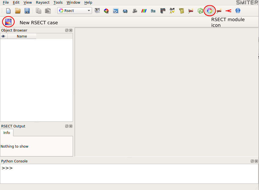
Fig. 4.111 SMITER interface and RSECT module icon.

After RSECT module icon is clicked, a new toolbar appears on the screen, where we can click on the Case icon to start the creation of a new RSECT case. After clickng this icon, a new case dialog appears on the screen. Dialog window is shown on a figure below.

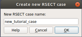
Fig. 4.112 New case dialog window.

With Create new RSECT case window, the user can manage the name of the new case. The default location of output is ~/rsect-compute, if user would like to change the location of output files, this can be done in Edit case section. After clicking OK button on the dialog window, Raysect section appears in the Object Browser on the right, as shown on a figure below.

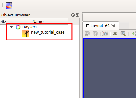
Fig. 4.113 New case in Object Browser.

4.24.1.1. Importing data

After that, Import mesh window is shown. With that dialog window one can add objects to the virtual environment. We can see the Import mesh dialog window and the workflow of creating the environment on a figure below.

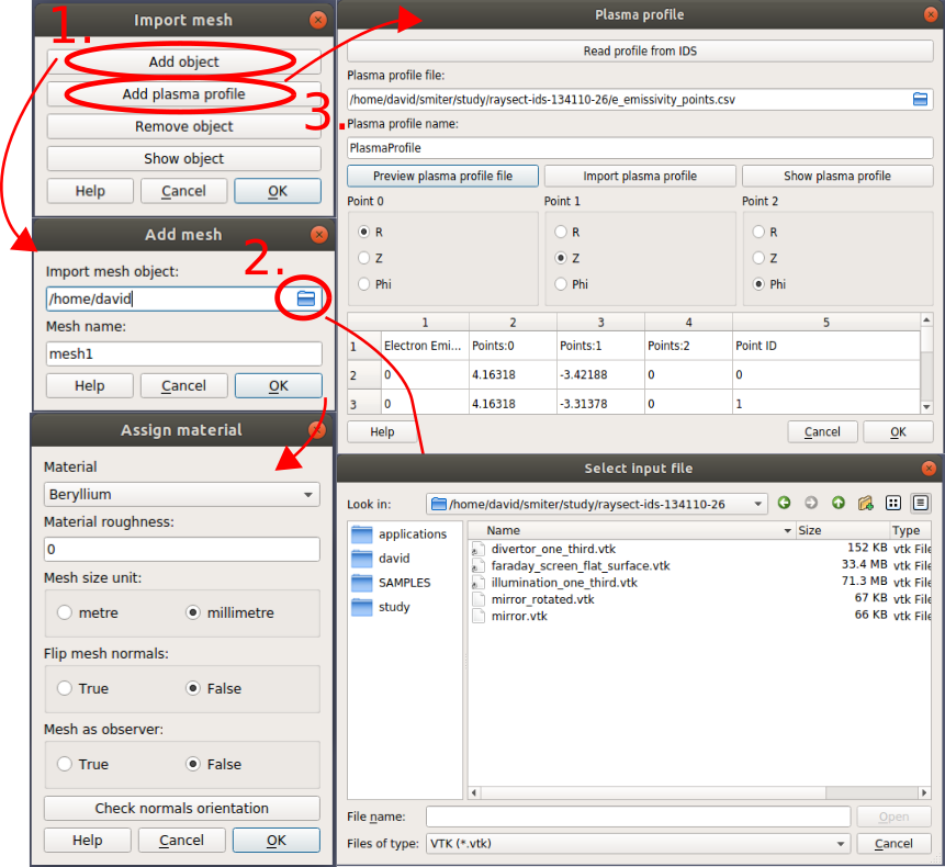
Fig. 4.114 Importing case objects workflow.

With this dialog window, case meshes can be imported to the case. As shown on the figure above, we first click on Add object button, and then Add mesh dialog appears on the screen. With clicking on the folder icon, the file select dialog window opens. After navigating to the mesh file location, we select the mesh file and click on the open button. Then we name the imported mesh. After clicking the OK button, Assign material window pops up, and from the drop down menu we select the material properties of the object. In the example case, Beryllium is selected as the mesh material. We also have to define the mesh units. Example meshes are in millimetres, as we selected. The normals of the objects, on which we would like to measure power emission, have to be facing the emission source. For objects, used in this tutorial, we flip the normals according to the table below. If we are not sure, whether the normals have to be fliped, we can check their orientation by pressing Check normals orientation button. To select the mesh as a mesh camera object, we have to make sure, that we checked the mesh as an absorber. We repeat this process for every mesh, which we would like to add to our case. For the example case, files in the table below are selected with perscribed properties.

Table 4.4 Rendering times with different number of cores

File name	Size units	Flip normals	Observer	Material
faraday_screen_flat_surface.vtk	millimetre	False	True	Beryllium
illumination_one_third.vtk	millimetre	False	True	Beryllium
mirror.vtk	millimetre	False	False	Perfect reflecting
mirror_rotated.vtk	millimetre	True	False	Perfect reflecting

To add the plasma source to the case we select Add plasma profile button. First Plasma profile dialog pops up, and we can select the plasma profile file, ids_134110_21.csv. Than we click on Import plasma profile button, which shows us the plasma profile folder preview. Electron emissivity, transformed in specific power in units W/m^3 is mapped in a rectangular grid. The location in the coordinate system is perscribed with coordinates, named Point:0, Point:1 and Point:2. Those coordinates present the R, Z and Phi coordinates of our data. We only have to connect the correct columns to the correct value in the coordinate system. For the example case, values are correctly set by default. Then we click on Show plasma profile button and the profile should appear in the window.

To add plasma profile we can also click on Read profile from IDS. New window pops up, like shown on a figure below. In that new window we type in the unique Shot and Run number. For this tutorial we set Shot = 134110 and Run = 26. User and device places should be already occupied with correct settings.

To get ids files you have to go to the terminal window and type:

cd ~/smiter/study/imas
make

This should make ids files in ~/public/imasdb/smiter/3/0.

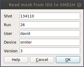
Fig. 4.115 Read profile from IDS.

After clicking OK button, user should wait for message window on figure below. After that, we can go to the Objrect browser and with right click on profile object we can than select Show plasma profile to see imported profile.

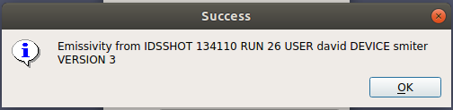
Fig. 4.116 Profile imported message.

We can also click on Show object button and select the objects in the Object Browser, which we would like to see. After we show the object, we can make sure that their position is correct and that scaling is correctly done. For tutorial case, we should see our case composition like it’s shown on a figure below.

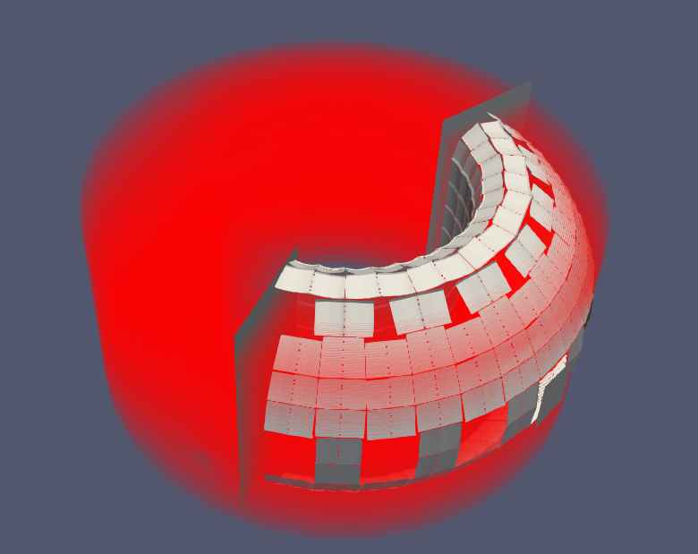
Fig. 4.117 Case objects composition with plasma source.

In case we would like to add some more objects or the plasma source to the case, we can right click on the case in Object browser and select the Add object or Add plasma option. Other options are shown on a figure below.

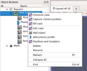
Fig. 4.118 Right click on case options.

With all that done, case objects should be in Object browser as shown on a figure below.

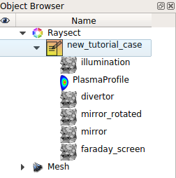
Fig. 4.119 Case objects in Object browser.

To show the object, we can right click on the object in the object browser and select the Show object option.

4.24.1.2. Settings

After checking if the meshes and the plasma source are correctly sized, we have to set the properties of analysis. First, we click the OK button on Import mesh dialog, which hides, and then Set case settings dialog appears on the screen. In that dialog we have two buttons, one is for showing the case objects, and the other is for the case settings. The dialog can be seen on a figure below.

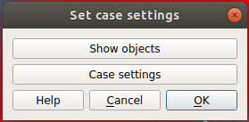
Fig. 4.120 Case settings.

If we click Show objects button, we can use the same procedure as described above. On the other hand, if we click Case settings button, a new RSECT case property dialog appears. The dialog is shown on a figure below.

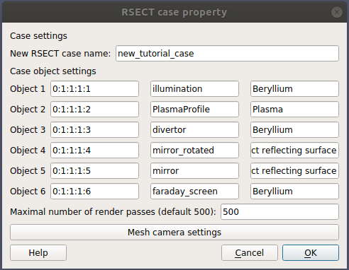
Fig. 4.121 Case settings.

This dialog shows us the case objects and we can set the maximal number of render passes. We also have to click on Mesh camera settings, to set the properties of the mesh observers (only if one of the meshes is set to observer). A new dialog appears and gives us options to set the surface offset, pipeline, sampler, number of bins, minimal and maximal wavelength. Dialog window is shown on a figure below.

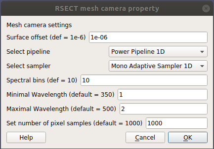
Fig. 4.122 Mesh camera property window.

Case properties can be changed by right clicking on the case in Object browser and then selecting Edit case, which opens RSECT case property dialog, or by clicking on Pipelines and Samplers which opens a dialog, shown on a figure below.

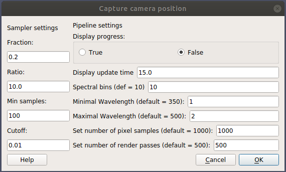
Fig. 4.123 Pipelines and samplers property window.

For the tutorial case, we used the settings, which are shown on figures above. After that, we head to the case in the Object window and with the right click on case we select Compute case.

After clicking compute case, the computing process should begin. In the terminal window, computing output should appear. An example is shown on a figure below.

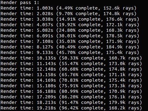
Fig. 4.124 Computing raysect case.

When computation is finished, you should be able to see this message in RSECT Output:

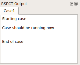
Fig. 4.125 Computing raysect case.

The output file in .vtk format is saved at location, which we defined in the first step of creating a new RSECT case. We can see the output in SMITER module ParaVIS. The example results can be seen on a figure below.

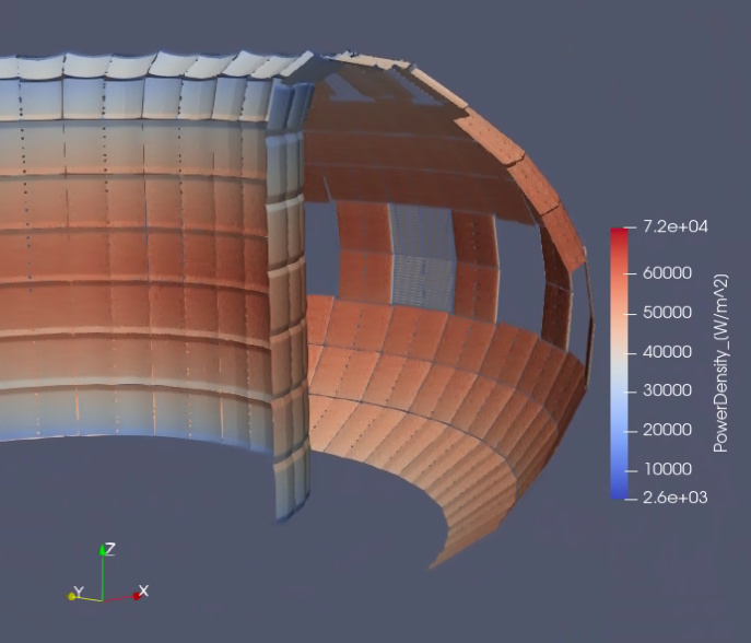
Fig. 4.126 Rsect tutorial case results.

Used color scheme is set to Rainbow Blended Grey for better representation.

4.24.2. Example with camera observer

With camera as observer we calculate the power that is observed thorugh the Pinhole camera set and oriented in a specific point in the virtual environment. We set the environment as we set it in the Mesh as observer example above. The only difference is that we never set a mesh as the observer. After we show all environment objects, we can position the camera. Positioning can be done manually with a mouse, or we can use Paraview options, as shown on a figure below.

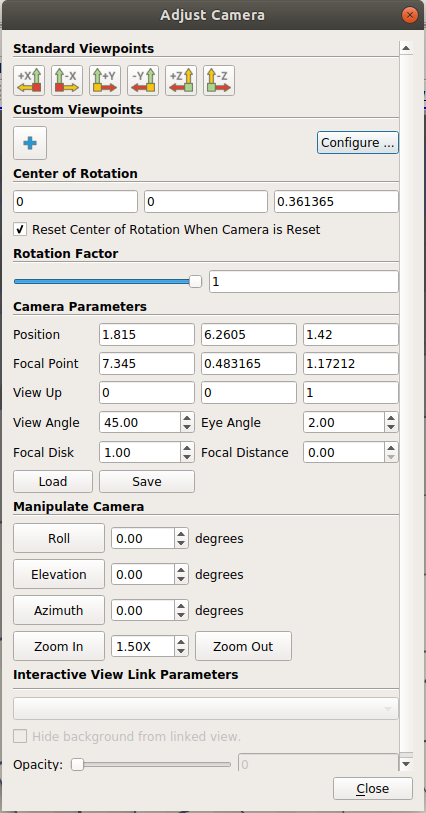
Fig. 4.127 Positioning the camera.

After we are satisfied with the camera positioning, we have to capture the camera position. This can be done with the right click on the case in Object browser and with selecting Capture camera position option.

After that a dialog appears, as shown on a figure below. In that dialog we can set some camera properties like number of pixels in X and Y direction, camera view angle, pipeline and sampler, and some other parameters. We can also change them in Pipelines and Samplers dialog mentioned above.

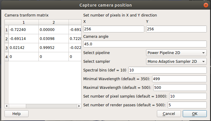
Fig. 4.128 Setting camera properties.

After all settings are set to the desired value, we can run the case with Compute case option after right clicking on the case. After all meshes are imported to the case and module starts the calculation process, Matplotlib window should appear on the screen, which will be updating its image. The image is tilted 90 degrees, but the final result should be ok. The output file is in a .csv format and can be presented in Paraview using Table to Points filter. Results of this example are shown on a figure below.

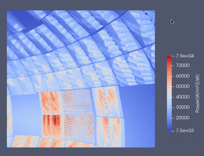
Fig. 4.129 Results of observing ITER reactor through camera.